Module 14. Learning from Feedback: RLHF, DPO, RLOO, and GRPO

Modern LLMs · Module 14 lecture · revision 2026.10.28

What this module is about. Module 13 taught a model to imitate demonstrations. That is enough when the target behaviour can be expressed as a strong reference answer. Many alignment goals are different: two responses may both be valid yet differ in usefulness, calibration, tone, or safety. Other tasks admit a direct signal from unit tests, a theorem checker, a simulator, or an interactive environment.

A comparison tells us which response is preferred; a checker reports an outcome for a task. Neither signal specifies how the model should learn from it. We will develop three routes: fit a separate evaluator, turn preference pairs directly into a training loss, or compare several fresh responses to the same prompt. The method names will become useful once these choices are clear.

The module keeps an engineering perspective. We will identify the signal consumed by each method, the models and data it requires, what its equations estimate, and why rollout generation can cost more than the parameter update itself.

Further study. The module is self-contained. The author's companion course RL for LLM develops policy gradients, reward models, PPO, DPO, RLOO, GRPO/RLVR, interactive environments, rollout infrastructure, and reward hacking in substantially greater depth.

Prerequisites. You should be comfortable with SFT from Module 13, the parameter-state memory estimates used in Modules 9 and 13, and the prefill/decode distinction from Module 10. Everything required for the derivations below is restated here, so the module remains self-contained. Reading routes. On a first pass, follow §§1, 3–7 and 9: identify the feedback signal, then trace how it changes the probability of an answer. In §8, focus on the data each method needs. Use §§10–11 to interpret the costs, then read §15 on verifiable rewards and checker limitations. Run §14 and answer Q1–Q4 in §18; Q5 follows the reference discussion in §17. On a second pass, work through the DPO derivation, the weighting and bias questions in §§9 and 12, and the projects in §19. Treat §§2, 8 and 16–17 as a reference map; learning the method names can wait until the mechanics are clear.

---

1. The signal changed: from imitation to judgment

A demonstration answers a concrete question: what response should the model imitate in this context? Preference data answers a different one: which of these responses should the model move toward?

That difference matters whenever there is no canonical target. Suppose two explanations are factually sound. One is concise and directly addresses the user's misconception; the other is more complete but spends a paragraph on background. A supervised dataset must choose one text as the target. A preference dataset can preserve the comparison without pretending that the winner is the only acceptable continuation.

There is a second source of supervision that is particularly important for reasoning. A completion may be checked by unit tests, a symbolic verifier, an exact answer, or the terminal state of an environment. In that case the feedback need not express a human taste at all. It is a measurable outcome.

A policy is the trainable model viewed as a distribution over answers. We write $\pi_\theta(y\mid x)$ for the probability of completion $y$ given prompt $x$ and parameters $\theta$. A sampled response, its context and its feedback form a trajectory; producing it is a rollout. In a noninteractive task, one complete answer can be the whole trajectory. “Online” means that training collects new data as the policy changes; it does not mean an internet connection is required.

The source of feedback and the timing of data collection are separate choices. Human or model judgments and programmatic checks can be applied to stored responses or to newly collected ones. We will contrast two common workflows.

• Offline preference optimization consumes a fixed collection of pairs or labels. The original DPO recipe is an example.
• Online reinforcement learning samples fresh completions from the policy being trained, scores them, and updates the policy from those trajectories. PPO, RLOO, and GRPO belong here.

Offline training is easier to reproduce and does not pay for generation at every optimizer step. Its blind spot is distribution shift: the dataset reflects policies that produced the stored answers, not necessarily the policy after several epochs of training. Online RL follows the moving policy distribution, but the system must now generate, score, transport, and sometimes discard a large number of trajectories.

The rest of the module can be read as three different answers to one design question: what mathematical object should a comparison become? A scalar reward model, a pairwise classification loss, or a relative advantage inside a group of sampled completions.

Keep the objective separate from the collection procedure. We study the original fixed-pair DPO recipe, but one can collect fresh preference pairs between DPO rounds. Likewise, a verifier defines where rewards come from, not which optimizer or group estimator must consume them.

2. From reward modelling to environment-scale RL

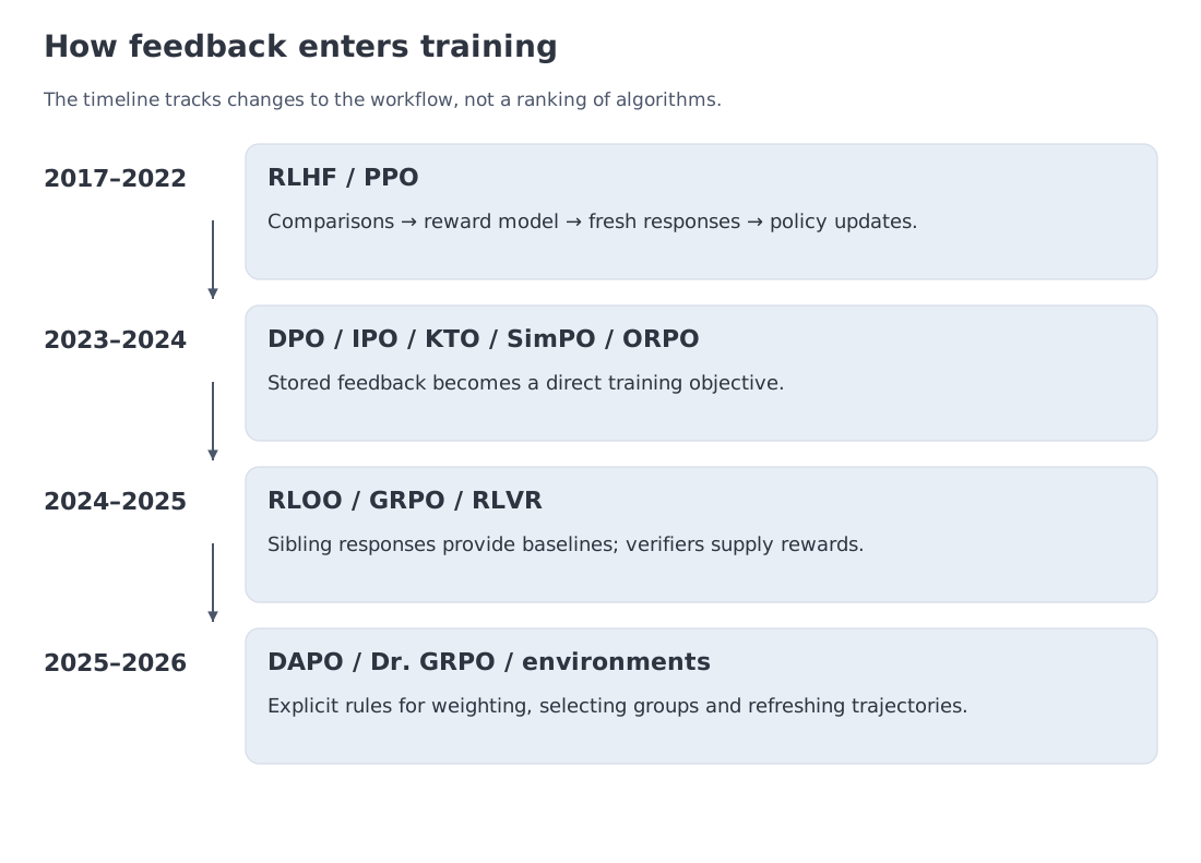
The modern pipeline did not appear all at once.

Christiano et al. (2017) showed how human comparisons could train a reward model for an agent. InstructGPT (2022) adapted the pattern to language models: supervised fine-tuning produced an initial assistant, a reward model learned from ranked answers, and PPO optimized the assistant while a KL term limited drift from the reference policy.

DPO (2023) removed the online RL stage for a particular class of preference objectives. By expressing the optimal reward through a ratio between the trained and reference policies, it turned the problem into a supervised pairwise loss.

By 2024, work was moving in two useful directions. IPO, KTO, SimPO, and ORPO explored alternative direct losses and data contracts. RLOO and GRPO revisited lightweight policy-gradient methods that construct baselines from multiple answers to the same prompt instead of training a separate critic.

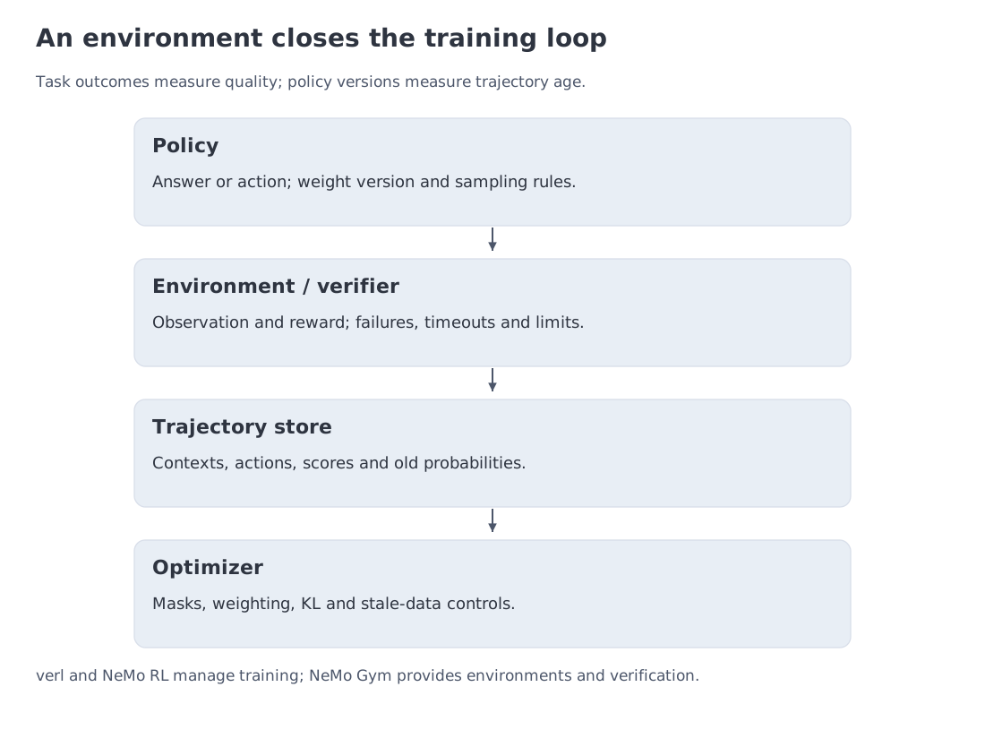
The open releases around DeepSeek-R1, DAPO, and Dr. GRPO in 2025 made verifier-based RL a central topic in reasoning-model research. The next step was architectural rather than merely algorithmic. By 2026, open stacks such as verl, NeMo RL, and NeMo Gym expose rollout workers, interactive environments, asynchronous queues, and trajectory-freshness controls as first-class components.

This is the important historical shift. Post-training is no longer well described as “run PPO once after SFT.” For agents and long reasoning tasks it increasingly resembles a distributed data-generation system in which the optimizer is only one stage.

3. Three old ideas that organize the new vocabulary

Preference optimization becomes easier to reason about when it is anchored to three classical constructions.

Bradley–Terry: pairwise choice from a score difference

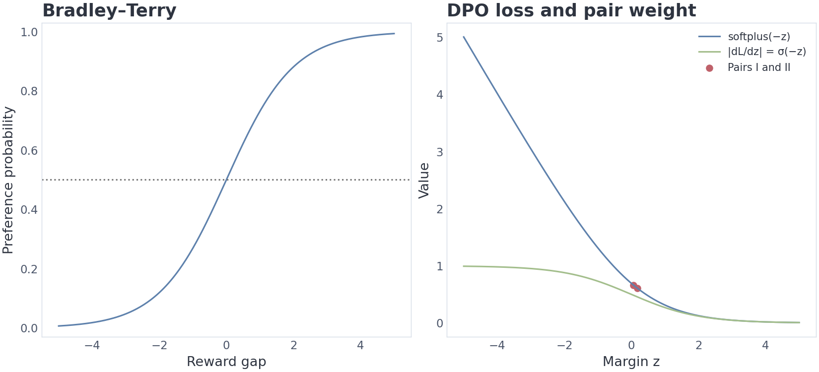
Assign each item a latent scalar score. The Bradley–Terry model writes the probability that item $i$ beats item $j$ as

$$P(i\succ j)=\sigma(s_i-s_j).$$

In RLHF the items are completions and the score is a learned reward. The standard reward-model loss,

$$\mathcal L_{\mathrm{RM}} =-\log\sigma(r_w-r_l),$$

is therefore logistic pairwise modelling, not an LLM-specific invention.

Here $\sigma(u)=1/(1+e^{-u})$ is the sigmoid, which maps a real score gap to a probability between zero and one. Subscripts $w$ and $l$ denote the preferred and rejected answers. Rejected means that the answer lost this comparison; it need not be factually wrong.

REINFORCE: reduce variance without changing the expectation

Let $J(\theta)$ be the expected reward under parameters $\theta$. For a one-step task, $J(\theta)=\mathbb E_{s,a\sim\pi_\theta}[R]$; in a multi-step task, $R$ denotes the future return. The score-function estimator gives

$$\nabla J(\theta) =\mathbb E\left[R\,\nabla\log\pi_\theta(a\mid s)\right].$$

Its variance can be reduced by subtracting a baseline that does not depend on the sampled action:

$$\nabla J(\theta) =\mathbb E\left[(R-b)\,\nabla\log\pi_\theta(a\mid s)\right].$$

RLOO forms $b$ from the other completions sampled for the same prompt. GRPO uses statistics of the entire group. The latter is convenient, but it is not automatically an unbiased substitute for a value function.

In these equations, $s$ is the context before an action, $a$ is the sampled action and $R$ is its reward. An action can be a complete answer or one token; in the latter interpretation, the context includes the generated prefix. The residual $A=R-b$ is called an advantage. Treat the baseline as a constant when taking this policy gradient. Rewards of the other responses provide an action-independent baseline when responses are conditionally independent draws from the same frozen sampler for that prompt.

Prospect theory: utility relative to a reference point

Human judgments are often asymmetric around a reference point: gains and losses of the same magnitude need not have the same subjective effect. KTO uses this perspective to learn from individual desirable and undesirable examples rather than explicit pairs.

These three ideas give us three different geometries: pairwise score gaps, policy-gradient advantages, and utility measured relative to a reference point.

Further study. The full DPO derivation, maximum-entropy interpretation of the KL term, and PPO mechanics are developed in RL for LLM, Modules 7–8. The information-theoretic role of KL regularization is covered in Information Theory for ML, Module 8.

4. Classical RLHF as an algorithmic contract

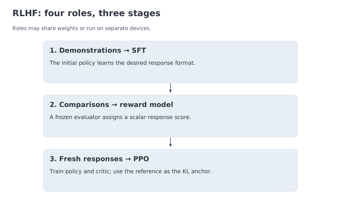
RLHF means reinforcement learning from human feedback. Let $\pi_{\mathrm{ref}}$ denote the policy obtained after SFT.

Stage 1: supervised fine-tuning. Demonstrations move the base model into a useful response distribution.

Stage 2: reward modelling. For prompt $x$, annotators compare a preferred completion $y_w$ with a rejected completion $y_l$. A reward model $r_\phi$ is trained with

$$\mathcal L_{\mathrm{RM}} =-\log\sigma\left(r_\phi(x,y_w)-r_\phi(x,y_l)\right).$$

Stage 3: policy optimization with PPO (Proximal Policy Optimization). The current policy samples completions and is optimized against the learned reward while remaining close to the reference:

$$\max_\theta\; \mathbb E_{x,\,y\sim\pi_\theta} \left[r_\phi(x,y)\right] -\beta\,\mathbb E_x\!\left[\mathrm{KL}\!\left(\pi_\theta(\cdot\mid x)\|\pi_{\mathrm{ref}}(\cdot\mid x)\right)\right].$$

The positive coefficient $\beta$ sets the penalty for departing from the reference, and $\mathbb E_x$ averages over training prompts. Recall the KL definition from M13; the direction used here is

$$\mathrm{KL}(\pi_\theta\|\pi_{\mathrm{ref}}\mid x) =\sum_y\pi_\theta(y\mid x)\log\frac{\pi_\theta(y\mid x)}{\pi_{\mathrm{ref}}(y\mid x)}.$$

The sum runs over complete responses, with the log ratio averaged under the current policy. This is a soft incentive to stay near a fixed reference, not a bound on the size or speed of each update. PPO also modifies the objective relative to the policy that collected the current batch; §9 treats that mechanism separately. Neither mechanism repairs an incorrect reward or guarantees safe behaviour.

The critic predicts expected future reward from the current context. Comparing the observed return with this prediction helps estimate advantage: how much better the action turned out than expected. The reward model has a different role: it scores a response using learned preferences.

The canonical pipeline contains four logical roles: policy, reference policy, reward model, and critic/value model. A production implementation may share backbones, shard states, quantize frozen models, or place the roles on separate machines. “Four models” is therefore an algorithmic description, not a claim that four independent full checkpoints must remain resident on every accelerator.

5. Worked example A: invert a Bradley–Terry model

Write $\Delta r=r_w-r_l$. Then

$$P(y_w\succ y_l)=\sigma(\Delta r).$$

A gap of 1 corresponds to roughly a 73% preference probability under this model. A gap of 2 raises it to about 88%. The units are not universal; the scale is set by the model and its regularization.

The equation can also be inverted. If one completion wins 75% of comparisons, the corresponding logit is

$$\Delta r =\log\frac{0.75}{0.25} =\log 3 \approx1.099.$$

This does not reveal an objective human utility. It maps an empirical win rate into the coordinate system of a logistic comparison model. That coordinate system will reappear in DPO, where $\beta$ controls the scale of policy log-ratios.

6. DPO: eliminate the explicit reward model

DPO (Direct Preference Optimization) starts from the KL-regularized objective in §4. For that objective, the optimal policy has the form

$$\pi^*(y\mid x) \propto \pi_{\mathrm{ref}}(y\mid x) \exp\!\left(\frac{r(x,y)}{\beta}\right).$$

The proportional weights become probabilities after division by the normalizing sum

$$Z(x)=\sum_y\pi_{\mathrm{ref}}(y\mid x)\exp\!\left(\frac{r(x,y)}{\beta}\right).$$

Assume this sum is finite and the reference assigns positive probability to the responses under consideration. Rearranging then gives

$$r(x,y) =\beta\log\frac{\pi^*(y\mid x)}{\pi_{\mathrm{ref}}(y\mid x)} +\beta\log Z(x).$$

The partition term depends on the prompt but not on the completion. It cancels in a pairwise reward difference. Substituting into Bradley–Terry yields

$$\mathcal L_{\mathrm{DPO}} =-\log\sigma\!\left( \beta\left[ \log\frac{\pi_\theta(y_w\mid x)}{\pi_{\mathrm{ref}}(y_w\mid x)} - \log\frac{\pi_\theta(y_l\mid x)}{\pi_{\mathrm{ref}}(y_l\mid x)} \right] \right).$$

The quantity

$$\hat r_\theta(x,y) =\beta\log\frac{\pi_\theta(y\mid x)}{\pi_{\mathrm{ref}}(y\mid x)}$$

is commonly called an implicit reward. The phrase is useful as long as its scope is remembered: DPO has not produced a standalone reward function that can score arbitrary model outputs independently. The reward is defined through two policies under the assumed preference model.

The original DPO recipe trains on fixed pairs without generating at each step. Precompute the reference log probabilities for those pairs and the reference checkpoint need not remain in the optimization process. Newly collected pairs require new reference values; changes to tokenization or the reference policy invalidate the corresponding cache. Refreshing the dataset therefore adds bookkeeping and scoring work rather than making caching impossible.

The implicit score can be evaluated on a new answer wherever both policies assign positive probability. It requires both policies, however; it is not an independently trained judge. A positive implicit reward gap describes ordering relative to the reference and does not establish answer quality beyond the comparisons used in training.

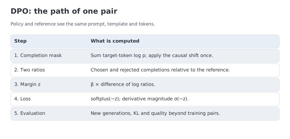
For a completion, $\log\pi_\theta(y\mid x)$ is the sum of $\log\pi_\theta(y_t\mid x,y_{<t})$ over its target tokens. As in M13, align the preceding-position logits with each target exactly once, then exclude prompt and padding positions. Both policies must use the same dialogue template, tokenization and end-of-answer convention. Otherwise their difference also measures a mismatch in representation.

7. Worked example B: read the DPO margin carefully

For pair I, the preferred response has policy and reference log probabilities $-12.0$ and $-13.0$, so its log-ratio is $+1.0$. The rejected response has $-11.5$ and $-10.8$, giving a log-ratio of $-0.7$.

With $\beta=0.1$,

$$z=0.1\,[1.0-(-0.7)]=0.170.$$

The pair loss and the derivative with respect to $z$ are

$$\mathcal L=-\log\sigma(0.170)=0.6118, \qquad \left|\frac{\partial\mathcal L}{\partial z}\right| =\sigma(-z)=0.4576.$$

For pair II, keep the policy values and use reference log probabilities $(-12.8,-11.65)$ for the preferred and rejected answers. The log ratios are $0.8$ and $0.15$, a gap of $0.65$. Thus $z=0.065$ and the derivative magnitude is 0.4838. At the decision boundary $z=0$, the magnitude is 0.5; for a misordered pair with $z<0$, it exceeds 0.5 and approaches 1 as $z$ becomes very negative. A near-boundary pair therefore pulls harder than an already well-ordered pair, while a strongly misordered pair receives an even larger local weight.

If pair I is evaluated with $\beta=0.5$, then $z=0.85$, the loss falls to 0.356, and $\sigma(-z)$ becomes 0.299. This number alone does not say that training has become weaker. The gradient with respect to model parameters also carries the factor $\beta$, and $\beta$ changes the scale at which policy movement is judged relative to the reference. In practice it should be tuned with KL drift, response quality, and the distribution of pair margins in view.

8. Direct preference losses differ by contract, not branding

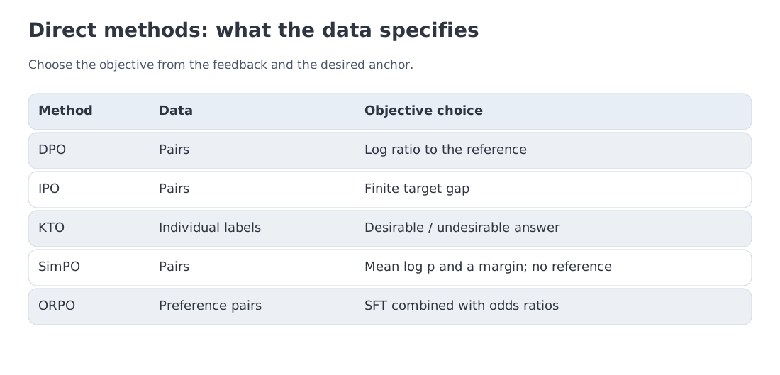
The family is easier to navigate if every method is described by the data it expects, the anchor it uses, and the margin it tries to create.

IPO: target a finite gap

Identity Preference Optimization (IPO) is derived as a special case of the broader $\Psi$PO framework. It replaces the unbounded logistic pressure of DPO with an objective that targets a finite preference gap. That can be useful when labels are noisy or many pairs are genuinely close.

The finite target is an inductive bias, not a free correction. A poor target can underfit strong preferences or encode the wrong calibration.

KTO: learn from desirable and undesirable examples

Kahneman–Tversky Optimization (KTO) removes the requirement that every label come as a pair. An example is marked desirable or undesirable and evaluated relative to a reference point.

A single-answer rating can be easier to collect because no alternative needs to be shown. What it omits is the identity of a comparison response. Neither one binary rating nor one binary pairwise choice directly specifies preference strength or a reason; those require additional annotations or explanations. The usefulness of pointwise feedback depends on negative-example quality, class balance and the reference point.

SimPO: a reference-free sequence reward

Simple Preference Optimization (SimPO) uses average sequence log probability as its implicit reward and adds a target margin. Length normalization replaces the sum of token log probabilities with their average, while the absence of a separate reference model reduces memory and compute.

Length normalization changes the incentive; it does not guarantee that response length will be neutral under every dataset and evaluation protocol.

Write $\bar\ell_\theta(y)=\log\pi_\theta(y\mid x)/|y|$ for a completion's mean token log probability. A SimPO pair then contributes $-\log\sigma(\beta[\bar\ell_\theta(y_w)-\bar\ell_\theta(y_l)]-\gamma)$, where $\gamma$ specifies the target margin. Ordinary autoregressive sampling follows the product of token probabilities; it does not rank complete answers by this average. Length normalization is therefore an objective choice whose effect must be checked on generated lengths and quality.

ORPO: preference alignment inside instruction tuning

Odds Ratio Preference Optimization (ORPO) combines the likelihood of the preferred response with an odds-ratio penalty for the rejected response. It is reference-free and is designed as a monolithic instruction-tuning objective rather than a separate alignment stage.

The simplified pipeline comes with tighter coupling. When results deteriorate, the supervised and preference components must be diagnosed together.

DPO remains a strong reproducible baseline. KTO is attractive for pointwise feedback, SimPO for a reference-free setup, ORPO for a single joint stage, and IPO when a finite target gap is a better model of the annotations.

9. RLOO and GRPO: construct a baseline from sibling rollouts

Offline pairs cannot follow the policy indefinitely. For verifiable tasks, it is often preferable to sample fresh completions from the current policy and score them immediately.

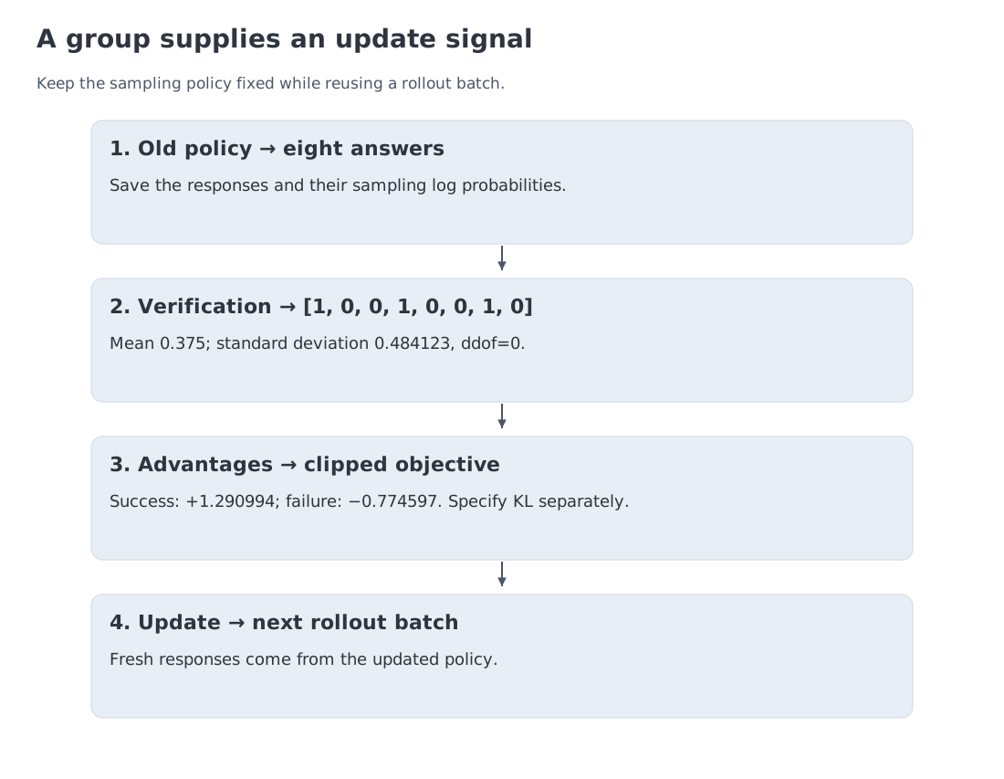
REINFORCE Leave-One-Out (RLOO) samples $G$ completions for one prompt. Completion $i$ uses the mean reward of the other $G-1$ completions as its baseline:

$$b_i=\frac{1}{G-1}\sum_{j\ne i}r_j, \qquad A_i=r_i-b_i.$$

Under the usual conditional-independence assumptions, the baseline does not depend on completion $i$ and preserves the expectation of the REINFORCE gradient.

Group Relative Policy Optimization (GRPO) instead standardizes rewards with statistics from the entire group:

$$A_i=\frac{r_i-\operatorname{mean}(r_{1:G})} {\operatorname{std}(r_{1:G})}.$$

The advantage is inserted into a PPO-style clipped objective, but no learned value model is required. GRPO is often associated with RLVR, although the reward may also come from a learned judge.

Take the binary reward vector

[1, 0, 0, 1, 0, 0, 1, 0].

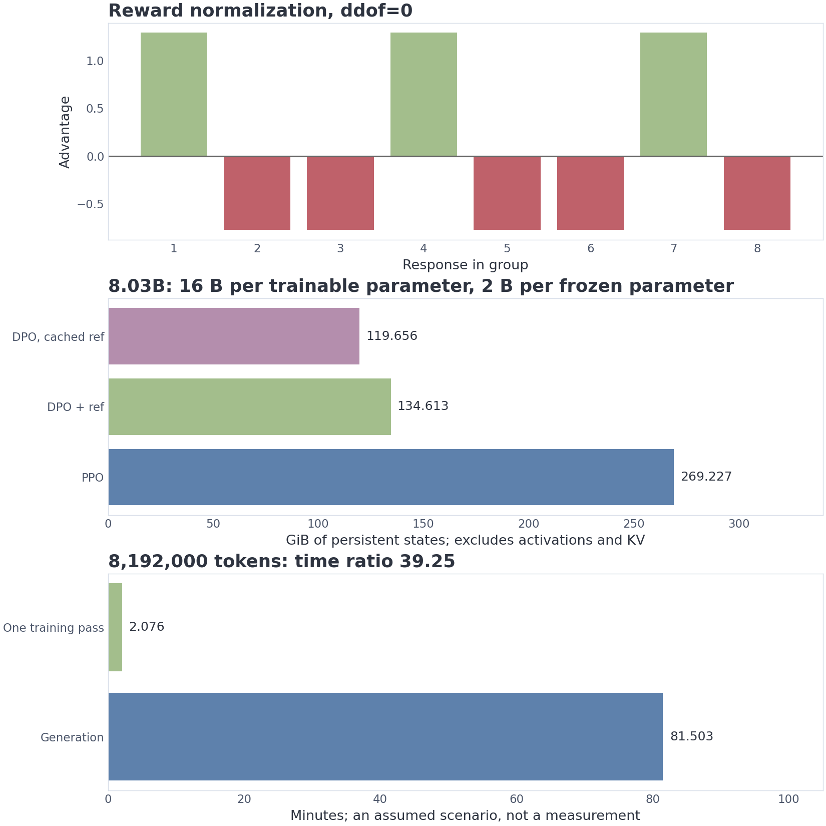
Its mean is 0.375 and its population standard deviation is 0.4841. Successful completions receive

$$A_+=1.291,$$

and unsuccessful ones receive

$$A_-=-0.775.$$

The advantages sum to zero. That is a within-group centering identity, not a proof that the estimator equals the true expected advantage. Because each sample contributes to the statistics used to normalize itself, group-relative methods can introduce difficulty- and length-dependent biases.

A group with identical rewards has zero variance. If rewards are Bernoulli with success probability 0.3 and $G=8$, the probability of an all-success or all-failure group is

$$0.3^8+0.7^8=0.0577.$$

Such a group contains no relative ranking signal. Skipping it, resampling it, or assigning zero advantages are explicit policy choices; adding epsilon to the denominator only prevents a numerical exception.

Our arithmetic uses the population standard deviation, ddof=0. Switching to ddof=1 multiplies the advantages by $\sqrt{(G-1)/G}$, changing the update scale at the same learning rate. Equal rewards produce zero policy-gradient advantages, but a separate KL penalty can still update the model. Dropping a group also changes the averaging denominator; collecting a replacement costs additional rollouts.

Turning an advantage into an update. Freeze the sampling policy $\pi_{\mathrm{old}}$ for a batch of trajectories. It is distinct from $\pi_{\mathrm{ref}}$: the former follows successive rollout batches, whereas the latter supplies a longer-term anchor. For completion token $t$ in answer $i$, define

$$\rho_{i,t}=\frac{\pi_\theta(y_{i,t}\mid x,y_{i,<t})} {\pi_{\mathrm{old}}(y_{i,t}\mid x,y_{i,<t})}, \qquad q_{i,t}=\min\!\left(\rho_{i,t}A_i,\, \operatorname{clip}(\rho_{i,t},1-\epsilon_{\mathrm{low}},1+\epsilon_{\mathrm{high}})A_i\right).$$

Maximize an average of $q$, or minimize its negative, treating the old probabilities and advantages as constants. For positive advantage, increasing the ratio past its upper threshold stops improving this term; negative advantage produces the corresponding limit on decreasing the ratio. Clipping shapes the objective. It does not guarantee that every probability ratio after an optimizer step stays inside the interval.

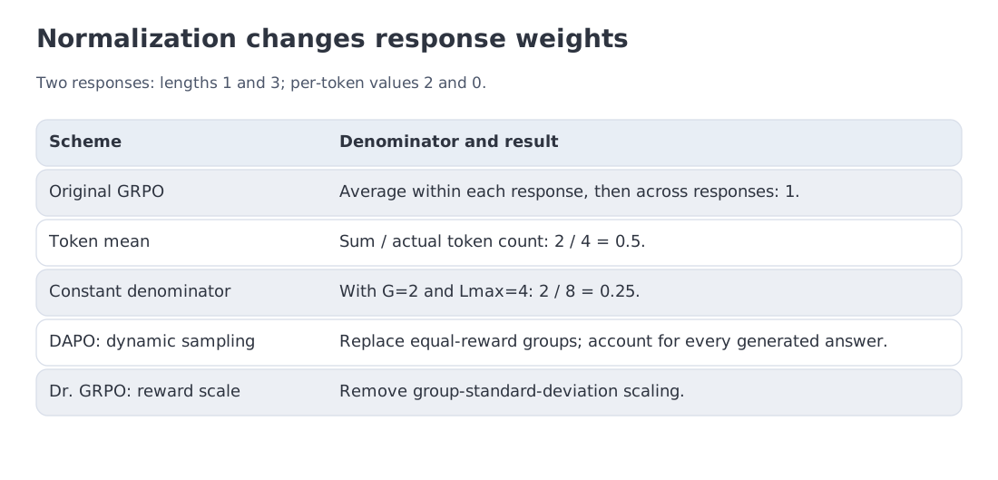
The denominator is part of the algorithm. Original GRPO averages tokens within each response, then responses: $G^{-1}\sum_i |y_i|^{-1}\sum_t q_{i,t}$. A token mean divides $\sum_{i,t}q_{i,t}$ by $\sum_i|y_i|$; the notebook's numerical example uses this normalization, as in that component of DAPO. If responses have lengths 1 and 3 and constant per-token values 2 and 0, these averages are 1 and 0.5 respectively. Padding enters neither sum. If KL regularization is used, specify its coefficient and normalization separately.

10. Worked example D: a deliberately simplified memory model

Assume an 8.03B-parameter model. Use 16 bytes per parameter for the teaching Adam stack: bf16 weights (2), bf16 gradients (2), an fp32 master copy (4), and two fp32 Adam states (4 + 4). A frozen bf16 copy costs 2 bytes per parameter. Other precision and optimizer choices change this accounting.

A trainable model then occupies

$$\frac{8.03\times10^9\times16}{2^{30}} =119.7\ \text{GiB},$$

while a frozen copy occupies 14.96 GiB.

For a transparent PPO teaching configuration, count two trainable full-sized networks—policy and critic—and two frozen ones—reference and reward model:

$$\frac{36\cdot8.03\cdot10^9}{2^{30}}\approx269.2\ \text{GiB}.$$

DPO with a resident reference policy uses

$$\frac{18\cdot8.03\cdot10^9}{2^{30}}\approx134.6\ \text{GiB}.$$

The ratio is exactly 2.00 under these assumptions, and the critic accounts for roughly 44% of the PPO total.

This is an anatomy diagram, not a cluster quote. It omits activations, rollout KV state, temporary buffers, parameter sharding, shared backbones, PEFT, optimizer variants, and distributed placement. A GRPO system may still need a reference model for KL, a sampling snapshot, and dedicated rollout workers.

For a fixed DPO dataset, cached reference log probabilities remove the frozen checkpoint from the optimizer phase. The persistent model-state budget then approaches the SFT case. That is a property of the offline workflow, not of every possible DPO implementation.

11. Worked example E: rollout generation can dwarf the update

Consider one illustrative RLVR batch:

• 256 prompts;
• 8 completions per prompt;
• 4,000 generated tokens per completion.

The rollout volume is

$$256\times8\times4000=8{,}192{,}000$$

tokens.

At 209.4 tokens/s on each of eight accelerators, generation takes

$$\frac{8{,}192{,}000}{8\times209.4} =4890.2\ \text{s} =81.5\ \text{min}.$$

Estimate one training pass with $6ND$ for an 8.03B model. At 990 TFLOP/s per accelerator and 40% MFU across eight accelerators, the estimate is $6\cdot8.03\cdot10^9\cdot8{,}192{,}000/(8\cdot990\cdot10^{12}\cdot0.4\cdot60)\approx2.076444$ minutes.

Compute the ratio before rounding either time; displaying six decimal places gives

$$81.502706/2.076444\approx39.2511.$$

Nothing in GRPO guarantees this number. It comes from the chosen completion length, throughput, model size, and utilization. What the example exposes is the possibility that autoregressive decode—not backpropagation—sets the wall-clock scale of RL.

That observation motivates four systems techniques:

1. faster and cheaper rollout inference;
2. adaptive allocation of rollout count and response length;
3. overlap between rollout generation and optimization;
4. explicit control of policy staleness in asynchronous training.

verl and NeMo RL both expose separated or asynchronous rollout/training architectures. The gain is not free: trajectories produced by older parameters become increasingly off-policy as they wait in queues.

Here 209.4 tokens/s is an assumed aggregate per-device rate at a chosen batching setup, not a promised per-user rate. The calculation counts generated tokens and one training pass over them. Prompt processing, prefill, reward and reference evaluation, extra optimization epochs and communication add work. Account for these separately before using the estimate to size a system.

12. What later GRPO variants are actually fixing

GRPO's adoption exposed several independent failure modes: groups with no relative signal, collapsing exploration, response-length bias, prompt-difficulty bias, and expensive sampling. Later methods should be read as targeted repairs, not as a single leaderboard sequence.

DAPO: a complete large-scale recipe

Decoupled Clip and Dynamic sAmpling Policy Optimization (DAPO) combines four mechanisms.

1. Clip-Higher sets a wider upper than lower ratio threshold, supporting exploration.
2. Dynamic Sampling discards equal-reward groups and continues collecting until enough informative groups fill the batch.
3. Token-Level Policy Gradient Loss changes the averaging unit so long and short completions contribute differently from response-level averaging.
4. Overlong Reward Shaping smooths the reward near the truncation boundary.

The published recipe also sets the explicit KL penalty to zero. That is an empirical system choice, not a general theorem that reference regularization is unnecessary.

Dr. GRPO: inspect the normalization itself

Understanding R1-Zero-Like Training argues that response-length and group-standard-deviation normalization can introduce optimization bias. Its Dr. GRPO variant removes parts of that normalization and improves token efficiency in the authors' experiments.

The paper also makes a broader methodological point: the base checkpoint already determines what behaviours RL can amplify. An “aha moment” observed during training should not automatically be interpreted as a capability created from nothing.

2025–2026: group-relative advantage under theoretical scrutiny

Recent analyses study systematic bias with respect to prompt difficulty and reinterpret GRPO as a contrastive objective. These results do not make GRPO useless. They replace an overly simple story—“the group mean is a free critic”—with a more accurate one: group-relative normalization is a practical estimator with identifiable inductive biases.

A serious implementation must document at least six choices:

• reward definition;
• treatment of zero-variance groups;
• averaging unit: prompt, completion, or token;
• KL placement and coefficient;
• freshness of rollout data;
• evolution of prompt difficulty and completion length.

A small exact example exposes one source of bias. Let $a$ be Bernoulli with $p=\sigma(\theta)$ and reward $a$. The true reward gradient is $p(1-p)$. Subtracting the full-group mean, which includes the sample itself, gives expectation $(G-1)p(1-p)/G$; a leave-one-out baseline preserves $p(1-p)$. At $p=0.3$ and $G=8$, these are 0.18375 and 0.21. This calculation does not divide by standard deviation; doing so introduces another dependence on the sampled group. The notebook enumerates all $2^8$ groups before comparing the result with simulation.

Dr. GRPO uses a constant token denominator $G L_{\max}$ and removes group-standard-deviation reward scaling. A constant denominator differs from both a response mean and a mean over the actual number of generated tokens. Consequently, “GRPO” alone is not enough information to reproduce a training run.

13. Level-one code: the numerical core

The following functions reproduce the module's frozen examples. They are intentionally smaller than a trainer: the goal is to expose the contract of each calculation.

import math
import numpy as np

def stable_sigmoid(x):
    """Numerically stable sigmoid."""
    x = np.asarray(x, dtype=np.float64)
    return np.exp(-np.logaddexp(0.0, -x))

def dpo_loss(policy_lp_w, policy_lp_l, ref_lp_w, ref_lp_l, beta=0.1):
    """DPO from completion-token log-probability sums."""
    if not math.isfinite(beta) or beta <= 0:
        raise ValueError("beta must be finite and positive")

    pw, pl, rw, rl = np.broadcast_arrays(
        np.asarray(policy_lp_w, dtype=float),
        np.asarray(policy_lp_l, dtype=float),
        np.asarray(ref_lp_w, dtype=float),
        np.asarray(ref_lp_l, dtype=float),
    )
    if not all(np.all(np.isfinite(v)) for v in (pw, pl, rw, rl)):
        raise ValueError("log probabilities must be finite")

    z = beta * ((pw - rw) - (pl - rl))
    loss = np.logaddexp(0.0, -z)
    local_slope = stable_sigmoid(-z)
    return loss, local_slope, z > 0

def grpo_advantages(rewards, *, on_degenerate="raise"):
    """Population normalization with explicit zero-variance handling."""
    r = np.asarray(rewards, dtype=np.float64)
    if r.ndim != 1 or r.size < 2 or not np.all(np.isfinite(r)):
        raise ValueError("rewards must be a finite one-dimensional group of size >= 2")

    if on_degenerate not in ("raise", "zeros"):
        raise ValueError("on_degenerate must be raise or zeros")
    std = float(r.std(ddof=0))
    if std == 0.0:
        if on_degenerate == "zeros":
            return np.zeros_like(r)
        raise ValueError("the group contains no relative signal")
    return (r - r.mean()) / std

def stage_memory_gib(n_params, stack):
    """Teaching estimate of persistent model states, excluding activations."""
    if not math.isfinite(n_params) or n_params <= 0:
        raise ValueError("n_params must be finite and positive")
    bytes_per_parameter = {"train": 16, "frozen_bf16": 2}
    return sum(bytes_per_parameter[kind] * n_params for kind in stack) / 2**30

ppo = stage_memory_gib(
    8.03e9,
    ["train", "train", "frozen_bf16", "frozen_bf16"],
)
dpo = stage_memory_gib(8.03e9, ["train", "frozen_bf16"])

np.logaddexp(0, -z) is the stable form of $-\log\sigma(z)$. local_slope is the derivative magnitude with respect to the scalar margin, not the norm of the parameter gradient. grpo_advantages forces the caller to decide what a zero-variance group means. stage_memory_gib states its limitation in the name and docstring: activations and rollout state are outside the model.

15. RLVR still obeys Goodhart's law

Reinforcement Learning with Verifiable Rewards (RLVR) replaces a subjective reward proxy with a programmatic checker. Unit tests, exact-answer matching, proof verifiers, and environment success conditions can provide unusually clean supervision.

“Verifiable” does not mean “unhackable.” The policy optimizes the checker that exists, not the intention behind it.

• An incomplete test suite may reward a brittle program.
• A parser may accept a special output format that bypasses the intended reasoning.
• End-result reward cannot distinguish a robust solution from a lucky guess.
• A hard length cutoff may create incentives to stop prematurely or fill the entire budget.
• Once easy prompts become all-correct, they stop contributing relative signal to group-based methods.

A mature RLVR dashboard therefore contains more than mean reward. It tracks completion length, zero-variance-group rate, policy entropy, verifier failures, held-out tests, and sampled trajectories reviewed by humans.

The boundary between SFT and RL is porous. High-quality rollouts may be recycled into a new demonstration mixture. Conversely, an SFT checkpoint becomes the starting policy for online RL. Strong post-training recipes alternate between these signals rather than treating them as mutually exclusive schools.

16. Three open patterns: RLAIF, multi-stage reasoning, and environments

Constitutional AI and RLAIF

Constitutional AI uses a written set of principles to scale supervision. In the supervised phase, a model generates an answer, critiques it against a selected principle, and writes a revision; the revised responses become fine-tuning data. In the RL phase, a model judges pairs, a preference model is trained from those AI labels, and the policy is optimized against it. This second stage is commonly called reinforcement learning from AI feedback (RLAIF).

AI feedback reduces the amount of human comparison data required. It does not reduce governance to zero cost. The constitution must be designed, the judge calibrated, systematic biases measured, and self-reinforcing failure modes audited.

DeepSeek-R1 as a public multi-stage recipe

DeepSeek-R1 documents four distinct stages:

1. cold-start SFT on a small collection of long reasoning demonstrations;
2. reasoning-focused RL with verifiable rewards;
3. rejection sampling followed by another SFT stage;
4. broader RL covering general helpfulness and safety objectives.

R1-Zero starts the RL stage directly from a base model. It demonstrates that large-scale verifier-guided RL can amplify reasoning behaviours without a preliminary SFT stage, while also reporting readability and language-mixing failures. Later analyses emphasize that the base model already contains much of the structure that RL selects and strengthens.

Interactive environments

A single-turn math problem can be represented by a prompt, a completion, and a checker. An agent using a browser, shell, or software tool moves through a sequence of observations and actions. The environment must execute tools, preserve state, return errors, and define success.

NeMo Gym treats an environment as a combination of data, agent harness, tools, and verification logic. NeMo RL and verl support multi-turn rollouts and separated generation/training systems. This is the operational meaning of environment-native RL: the environment is part of the training specification, not merely a final reward function.

When a proprietary model has no complete public post-training recipe, its behaviour cannot fill that evidential gap. Adjustable reasoning effort, hidden chains of thought, or strong tool use do not uniquely identify PPO, DPO, GRPO, distillation, or any particular mixture. Public behaviour should not be presented as evidence for an undisclosed algorithm.

17. How to read a post-training passport

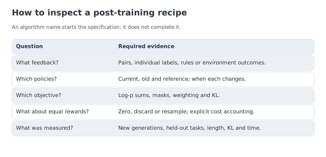
An algorithm name is not enough to reproduce or evaluate a post-training system.

Data and policy distribution

• Are the examples demonstrations, preference pairs, pointwise labels, or online trajectories?
• Which policy generated the completions: the current actor, an earlier checkpoint, or a stronger teacher?
• Are trajectories reused, and if so for how long?
• How are benchmark contamination and train/evaluation overlap controlled?

Reward contract

• Is feedback produced by humans, a learned judge, deterministic rules, tests, or an environment?
• Is reward assigned once per completion or along the trajectory?
• How are partial success, ambiguity, truncation, and invalid tool calls handled?
• What evidence establishes the accuracy of the verifier itself?

Optimization

• Is the algorithm offline, on-policy, or deliberately off-policy?
• Which roles are present: policy, old policy, reference, critic, reward model?
• Where is KL regularization applied?
• Is the loss averaged over prompts, completions, or tokens?
• What happens to zero-variance groups and extreme rewards?

Systems

• Are rollout and training workers colocated or disaggregated?
• Is the loop synchronous, one-step-off, or fully asynchronous?
• How is trajectory staleness bounded?
• What fraction of time is spent on decode, verification, communication, and optimization?

When these fields are absent, the honest conclusion is “the exact recipe is not disclosed.” Behavioural clues are useful for evaluation, not for reverse-engineering a training stack with certainty.

20. Key takeaways and sources

Distinguish the signals. Demonstrations specify a target. Preferences rank alternatives. Verifiers score outcomes. Specify the feedback format, data-collection procedure and update rule separately.

Classical RLHF. SFT feeds reward modelling, which feeds PPO under KL control. The four logical roles need not be four unshared full checkpoints in every implementation.

Bradley–Terry. $P(y_w\succ y_l)=\sigma(r_w-r_l)$. A 75% win rate maps to $\log3\approx1.099$ inside this comparison model.

DPO. The implicit reward is a current/reference policy ratio. The original DPO recipe is an offline pairwise method and does not require rollout generation or a separately trained reward model.

Direct variants. IPO targets a different margin geometry; KTO consumes pointwise desirable/undesirable labels; SimPO is reference-free and length-normalized; ORPO combines supervised likelihood and preference pressure in one objective.

RLOO and GRPO. Both compare sibling rollouts. RLOO uses a leave-one-out baseline. GRPO standardizes over the full group and removes the learned critic, but its estimator has identifiable bias and zero-variance cases.

The frozen scenarios. The persistent-state teaching model gives 269.2 GiB for PPO and 134.6 GiB for DPO with a resident reference. The rollout scenario gives a 39.3 ratio between generation and one training pass. Both are conditional calculations.

RLVR. A programmatic checker reduces subjectivity but remains a target that can be exploited. Verifier quality, length distributions, entropy, degenerate groups, and held-out tasks belong in the evaluation contract.

The systems transition. Modern RL post-training increasingly uses interactive environments, separated worker pools, asynchronous queues, and explicit freshness control.

Primary sources:

• Christiano et al., Deep Reinforcement Learning from Human Preferences — arxiv.org/abs/1706.03741
• Ouyang et al., Training Language Models to Follow Instructions with Human Feedback — arxiv.org/abs/2203.02155
• Rafailov et al., Direct Preference Optimization — arxiv.org/abs/2305.18290
• Azar et al., $\Psi$PO / IPO — arxiv.org/abs/2310.12036
• Ethayarajh et al., KTO — arxiv.org/abs/2402.01306
• Meng et al., SimPO — arxiv.org/abs/2405.14734
• Hong et al., ORPO — arxiv.org/abs/2403.07691
• Ahmadian et al., RLOO — arxiv.org/abs/2402.14740
• Shao et al., DeepSeekMath / GRPO — arxiv.org/abs/2402.03300
• Guo et al., DeepSeek-R1 — arxiv.org/abs/2501.12948
• Yu et al., DAPO — arxiv.org/abs/2503.14476
• Liu et al., Understanding R1-Zero-Like Training / Dr. GRPO — arxiv.org/abs/2503.20783
• Wu et al., It Takes Two: Your GRPO Is Secretly DPO — arxiv.org/abs/2510.00977
• Yang et al., Your Group-Relative Advantage Is Biased — arxiv.org/abs/2601.08521
• Bai et al., Constitutional AI — arxiv.org/abs/2212.08073
• Lambert et al., Tülu 3 — arxiv.org/abs/2411.15124
• NeMo Gym — docs.nvidia.com/nemo/gym
• NeMo RL — github.com/NVIDIA-NeMo/RL
• verl — github.com/verl-project/verl

Next: Module 15 studies reasoning models and test-time compute. Here we changed the policy; next we decide how much computation an already trained policy should spend on a particular request.

---

Landscape verified: October 11, 2026. Current claims were checked against primary sources; exact recipes for closed models are not reconstructed from external behavior. Teaching estimates for memory and time are reproduced by local calculations and apply only under the stated assumptions.