Module 3. The Basic Transformer
Modern LLMs · Module 3 lecture · revision 2026.10.25 · 11 October 2026
An embedding lookup gives a token the same starting vector wherever it occurs. A Transformer turns that vector into a contextual representation: one that depends on the surrounding tokens. This chapter follows the computation all the way to a distribution over the next token.
Bring matrix multiplication, matrix shapes, and embeddings from Module 2. Section 2 introduces tensors as multidimensional arrays. The chapter introduces the remaining concepts as they become useful. By the end, you will be able to trace the original encoder–decoder design and build a small causal language model.
Choose a reading route
- First pass: follow the information. Read §§1–12 in order; collapsed reference blocks can wait. In §2, focus on the input shape, and in §4.3, on what scaling accomplishes. Work through §4.5, then make sure the distinction between training and generation in §§11–12 is clear. Finish with §§16, 18, and 22. Save the longer code listings for the next pass.
- Second pass: make it run. Expand the shape reference in §2, revisit the argument in §4.3, and study §§13–15. Use the notebook in §20 and the exercises in §19 to reproduce the results and test the computation.
- Reference pass: locate a contract. Shapes are in §§2 and 15, masks in §5, normalization order in §8, and training versus generation in §§11–12. Section 17 collects common mistakes. If you can reconstruct the graph and answer §18 unaided, continue to Module 4.
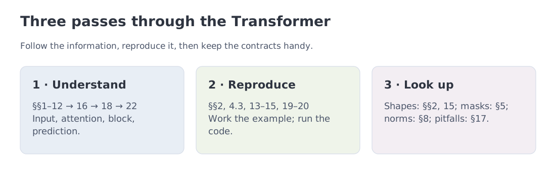 Start by following the information, then reproduce the computation, and keep the shape and mask contracts nearby as a reference.
1. Why the Transformer was needed
Start with the engineering problem rather than the equation. A model that translates a sentence, summarizes a document, or predicts the next token must combine two kinds of information at every position:
- the local content of the current token;
- information from other positions, where the useful positions depend on context.
In “the bank raised the rate,” the meaning of “rate” is constrained by “bank.” In code, a closing delimiter may depend on a construct opened many lines earlier. During translation, each target token must use both the generated target prefix and the complete source sequence.
A recurrent network computes state from state , creating a chain across positions. A Transformer instead uses attention: it builds a weighted mixture of vectors from accessible positions. When the requesting position and the vectors it reads belong to the same sequence, the operation is self-attention. A feed-forward network (FFN) then transforms each position’s features. Layers still depend on previous layers, but positions within a layer can be processed together.
Two mechanisms will make that computation respect sequence structure. A positional signal represents where a token occurs. A causal mask forbids a position from reading later tokens, which would reveal the answer during next-token training. Sections 3 and 5 make these ideas concrete.
The original Transformer paper (Vaswani et al., 2017) addresses translation. Its encoder turns the source text into contextual vectors, collectively called encoder memory. Its decoder builds the translation while reading both the available translation prefix and that memory. Attention that reads a different stream is called cross-attention. A decoder-only language model has no separate encoder: prompt and continuation occupy one sequence. Treat the next diagram as a map; the chapter will unpack its components.
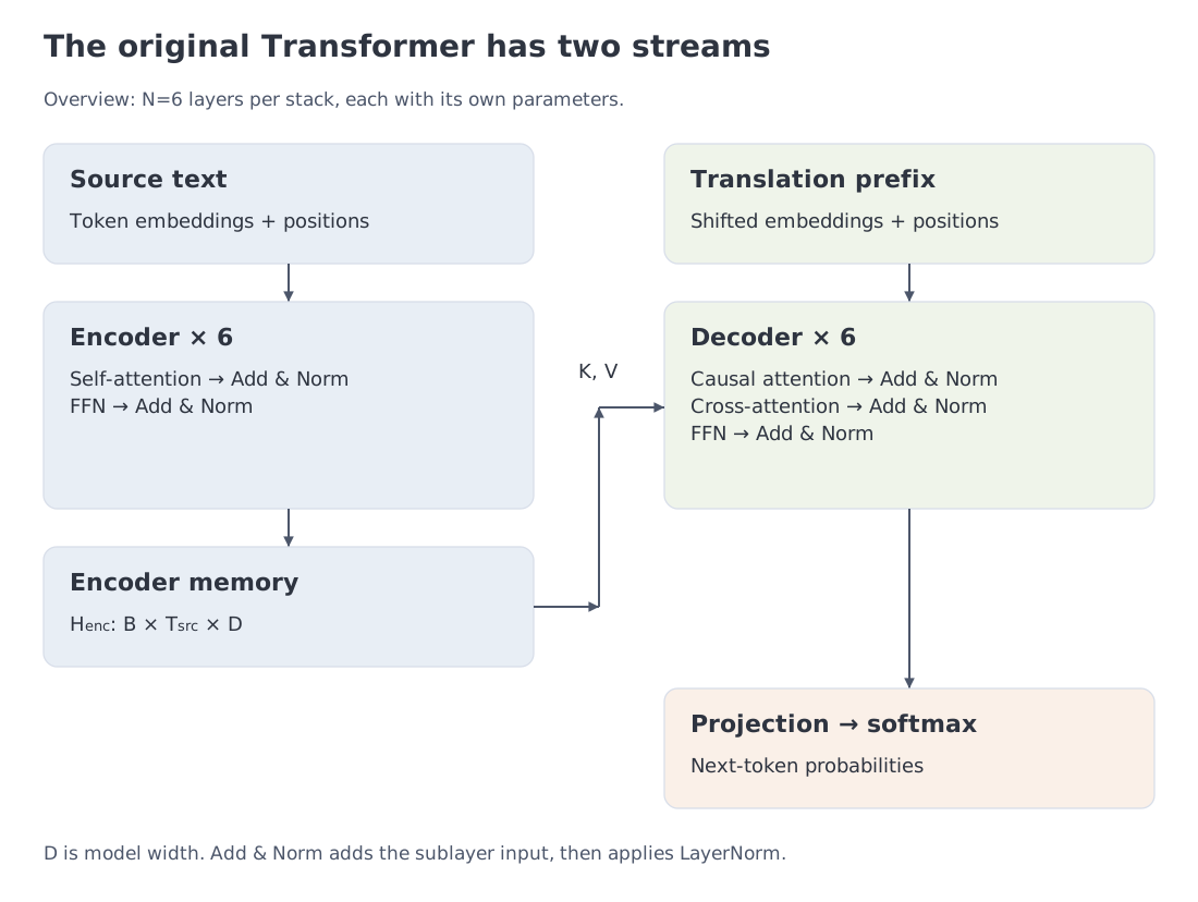 The source branch produces contextual vectors. The decoder uses them through cross-attention while building the translation. Sections 8–10 expand the sublayers and residual paths inside each branch.
1.1. Scope of this lesson
The immediate goal is to understand the basic computation. The following links are a map of later topics, not a list of prerequisites:
- Module 4 develops modern positional methods;
- Module 5 moves from MHA to GQA, MLA, and FlashAttention;
- Module 6 studies the modern residual block;
- Module 10 turns the autoregressive forward pass into efficient serving.
This chapter is self-contained. Those links deepen the subject but are not prerequisites for completing this lesson.
2. Notation and tensor shapes
Start with three axes. One token has features. A sequence has positions. A batch holds examples processed together. Their vectors form a tensor—a multidimensional array—of shape . Reading the axes as “example, position, feature” will prevent many shape errors.
For the first pass, keep in mind. Sections 4 and 6 introduce queries, keys, values, and heads; use the full index below once those concepts are familiar.
Full shape index — second pass and reference
| Symbol | Meaning |
|---|---|
| batch size | |
| sequence length | |
| , | number of queries and keys; usually equal in self-attention |
| number of features in the main representation stream | |
| number of attention heads | |
| , | key/query width and value width per head |
| hidden width of the FFN | |
| vocabulary size |
After embedding lookup,
For multi-head attention, it is convenient to expose the head axis:
Attention weights have shape
We will denote the value mixture produced by each head as :
The final axis of is the key axis. Softmax is applied there: for a fixed batch element, head, and query, key weights must sum to one. The final axis of instead has value width .
That is the first useful invariant. The second is that concatenated heads and the output projection must return to width , otherwise the result cannot be added to the residual stream.
2.1. The residual stream as the main route
The main representation keeps shape as layers refine it. This is the residual stream. Each sublayer computes an update of the same shape, and a residual connection adds that update to the input:
If the last dimension unexpectedly changes inside a basic block, that is almost never a subtle Transformer property. It is usually a shape bug or a missing output projection.
3. Step 1: tokens, embeddings, and positions
For this teaching model, IDs form the dense range , and the table has exactly rows. Real artifacts may distinguish defined IDs, the ID range, and allocated rows, as Module 2 explains.
A neural network does not receive a string directly. A tokenizer maps text to integer identifiers
An embedding matrix
acts as a learned lookup table. Row is the vector for the token at position . Batched lookup produces a tensor of shape .
The original architecture scaled token embeddings by and added a positional encoding:
The scale factor is not a universal law of every LLM; it belongs to the 2017 recipe. The important idea is the addition: token content and position enter the same residual space.
3.1. Why order vanishes without positions
Consider unmasked self-attention with no positional information. Permuting the input vectors permutes the output vectors in the same way. The mechanism sees a set of vectors and relations among them, but it does not know which vector came first.
For example, the vector associated with “dog” is unchanged when “dog bites person” becomes “person bites dog” under these assumptions; its output row simply moves. This property is permutation equivariance, not complete output invariance. A causal mask breaks that symmetry, so the argument applies specifically to unmasked attention without positional information.
3.2. Sinusoidal encoding in the original paper
Even and odd dimensions use sine/cosine pairs at different frequencies:
Here starts at zero, and indexes coordinate pairs from to for an even width. Small gives faster oscillations; large gives slower ones. This supplies several scales of variation. Being able to compute a positional code beyond the training lengths does not, by itself, guarantee useful model behavior there.
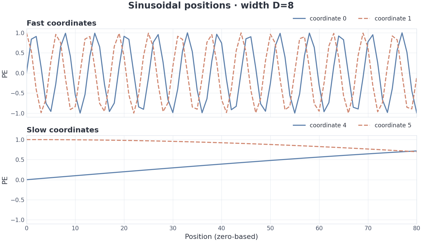 Four dimensions of one encoding. The high-frequency pair changes quickly from position to position, while the low-frequency pair supplies a slowly varying background.
This fixed formula makes a convenient starting point. Module 4 compares it with learned tables, relative biases, and RoPE rotations. For now, the key result is that a token vector carries information about both content and position.
3.3. A quick shape check
Let , , and :
token_ids:[2, 5];embedding(token_ids):[2, 5, 8];position_encoding[:5]:[5, 8];- after broadcasting and addition:
[2, 5, 8].
The positional table does not need a batch axis. The same coordinate is used for every item in the batch.
4. Step 2: scaled dot-product attention
Imagine one position requesting context. Its query describes what to match. Each available position supplies a key for matching and a value to contribute to the result. Attention turns query–key scores into weights and uses them to mix the values. One such computation is an attention head. The matrices , , and collect the respective vectors as rows. Queries and keys have width per head; values have width . There are queries and keys and values.
The computation for one head is
Softmax converts scores into nonnegative weights that sum to one. Here it operates separately for each query row, across the available keys. The transpose exchanges the final two axes so that the matrix product compares every query with every key. We will add masking after understanding this mixture.
It is useful to unpack the equation into three steps:
holds scaled compatibility scores, holds mixture weights, and contains the resulting vectors. The symbol in §6 will instead name the output projection matrix.
The matrix identity means, row by row,
Every query position receives a weighted sum of value vectors. Section 5 keeps the same computation but replaces with masked scores before softmax.
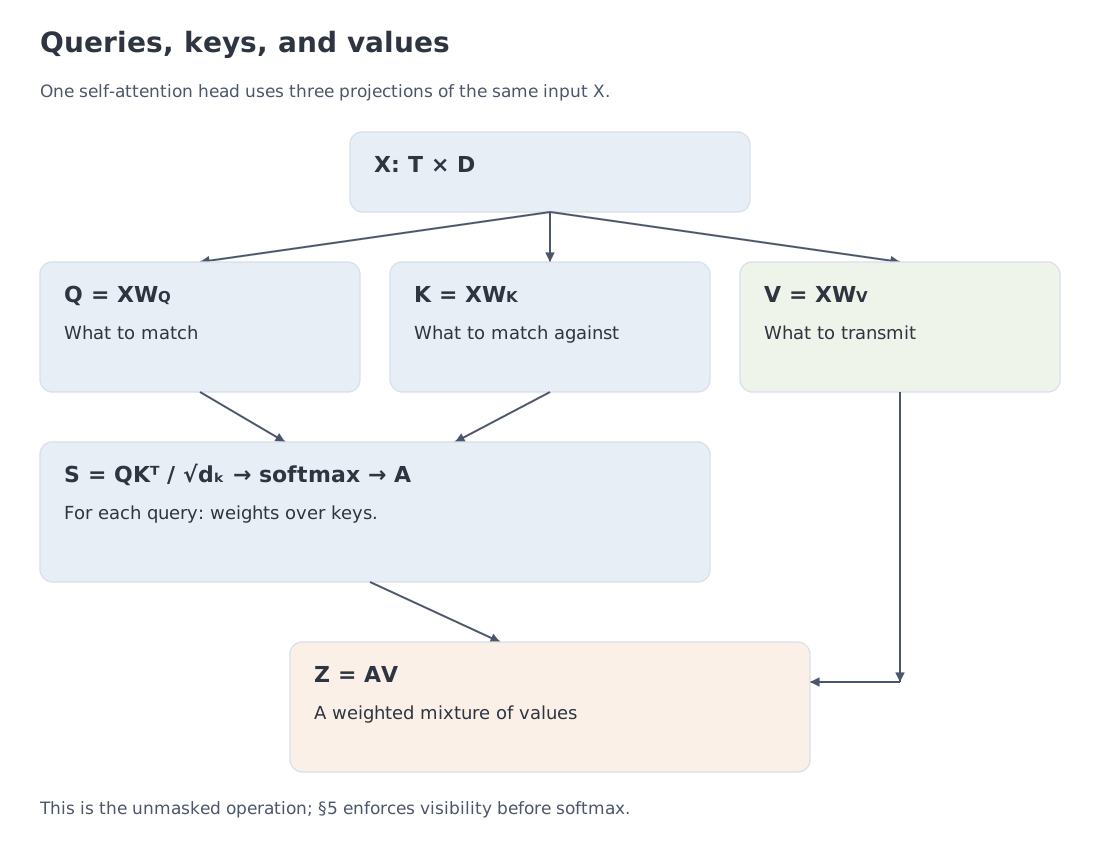 , , and are not three kinds of tokens. They are three learned roles assigned to representations. A table-lookup analogy helps as long as we remember that the query, index, and payload co-adapt during training.
4.1. Where , , and come from
In self-attention, all three tensors are linear projections of the same input :
For one head, we may write
The projections let the model learn different features for “what I am looking for,” “how I should be found,” and “what I transmit.” A token may have a key that is useful for a syntactic match while its value carries semantic or positional content.
In cross-attention, the sources differ:
Cross-attention changes where the vectors come from, while keeping the same scoring and mixing operation.
4.2. Why a dot product
Before scaling, the dot product of query with key is
The scores before softmax are attention logits. They are not yet probabilities: normalization turns each row into weights over keys. We will later use the same term for the model's output scores over vocabulary items.
A larger score receives a larger weight, all else equal. The sign alone does not establish relevance: softmax compares scores within a row. For nonzero vectors, cosine similarity is , which normalizes away their lengths. The dot-product score used here retains both magnitude and directional information.
4.3. Why divide by
Assume for intuition that coordinates and are independent, zero-mean, and unit-variance. Then
and under these simplifying assumptions,
The standard deviation grows like . Without scaling, wider keys can produce large logits, saturate softmax, make the distribution nearly one-hot, and leave small gradients for losing positions.
After division,
This is not a theorem about a trained network: learned coordinates are neither independent nor guaranteed to have unit variance. It is nevertheless an exact explanation of the natural scale and a phenomenon the notebook reproduces with random vectors.
4.4. Softmax and the correct axis
For query in unmasked attention,
Therefore
In code this is softmax(scores, dim=-1) when the final axis is . The wrong choice, such as dim=-2, may not raise an exception. It will normalize queries rather than keys. A row-sum assertion is therefore an essential unit test. Masked attention applies the same normalization to from §5.
4.5. Attention by hand: a complete numerical example
Use one head, three positions, and :
Scaled scores are
Apply the causal constraint: row 1 may read key 1, row 2 may read keys 1–2, and row 3 may read all three. Replace future-key scores with before softmax, making their exponentials zero, and normalize over the remaining keys. This gives
Let denote the head output. In matrix form , while each query row is
For this example,
The third row is especially useful to read in words:
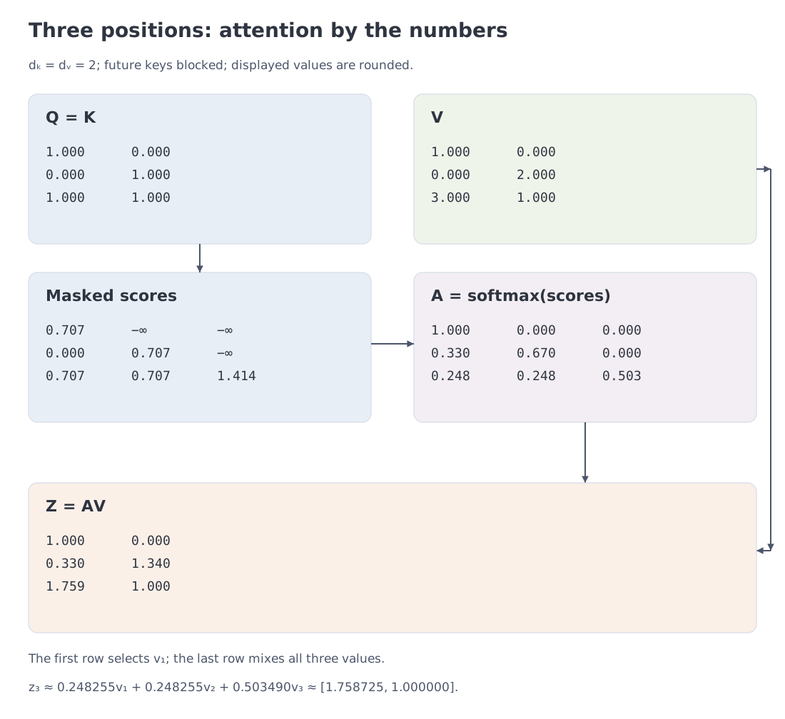 The full route through one head: compatibility matrix, future-token prohibition, key-wise softmax, and value mixing. The module notebook reproduces every number.
This example also exposes a crucial distinction: an attention weight is a routing coefficient, not a complete explanation of the model’s decision. A high weight says how much of a transformed value entered this local mixture. The result still travels through residual paths, other heads, FFNs, and later layers.
5. Masks: who is allowed to see whom
The word mask is used for two related but distinct objects: a Boolean visibility matrix and a numerical bias added to logits. Rather than hide the operation inside “scores + mask,” begin with a Boolean matrix
where means query is allowed to read key . Define masked scores directly:
Then
Because , forbidden connections receive zero weight. This is exactly the paper's prose description: illegal entries at the input to softmax are set to .
Implementations often express the same operation as
is a numerical bias constructed from , not a learned parameter. Allowed links receive 0 and forbidden links receive . A finite negative number only approximates this prohibition and does not resolve a row with no allowed keys (§5.6).
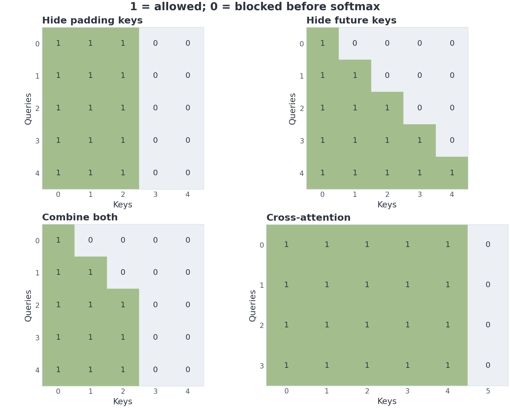 Padding-key and causal constraints can be combined. The fourth panel shows rectangular cross-attention. These plots mask keys; padded query rows are not independently suppressed.
5.1. Padding mask
Sequences in a batch have different lengths, but tensors are rectangular. Shorter examples are padded with PAD. Those positions contain no content and must not be used as keys. Query rows belonging to padding are normally excluded from the loss as well.
5.2. Causal mask
A decoder-only language model predicts token at position and must not use future context. Keys are allowed:
This is a lower-triangular pattern. It makes parallel training valid: all positions are computed in one forward pass, but each position receives only its admissible prefix.
5.3. Encoder self-attention
A classic encoder has no reason to hide right context. Every source representation may read the complete source sequence. Only padding needs to be masked.
5.4. Cross-attention mask
The number of target queries and source keys may differ. Decoder queries read encoder memory; padded source keys are hidden. A causal triangle over the source axis is normally unnecessary because the complete source is already available.
5.5. A common Boolean-mask trap
Even PyTorch uses two conventions: Boolean True allows a link in functional.scaled_dot_product_attention, but forbids one in MultiheadAttention.attn_mask. Our argument is named allowed, so True always permits a connection. A test checks that forbidden links receive zero weight.
5.6. A fully masked row
If a query is allowed to read no keys, the row does not define a probability distribution. A naive call such as
import torch

torch.softmax(torch.tensor([-float("inf"), -float("inf")]), dim=0)
# tensor([nan, nan])
produces NaN: subtracting the row maximum creates the indeterminate expression . A safe educational implementation must therefore expose an explicit policy:
error— the default: stop and surface a masking bug;zero— return zero weights and a zero output for that row when this is intentional, for example for a padded query excluded from the loss.
Under the zero policy the row sum of the weights is zero, not one. This is not an ordinary probability distribution; it is the contract “this query produces no attention output.” Silently substituting a uniform distribution or allowing NaN to propagate is incorrect.
6. Multi-head attention
One head produces one pattern of mixing weights. Multiple heads can produce different mixtures for the same position. Keep the notation explicit: are inputs before projection, while are projected vectors for head :
Self-attention uses ; cross-attention takes from the decoder and from the encoder. Every head sees the full input vector before projecting it to a narrower space.
Let be the number of heads. A common configuration uses
Concatenation then restores width .
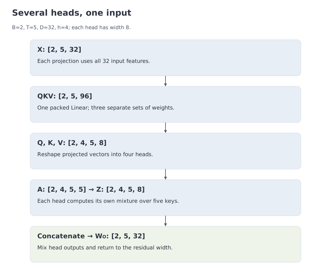 The three input projections are often computed by one packed linear layer, then reshaped by head. Independent attention results are concatenated and passed through .
6.1. Why several heads can help
Each head has different , , and projections. One head can become sensitive to local syntax, another to long-range matches, and another to separators or structure. That is a capacity, not a guarantee of clean, human-readable specialization. Heads may be redundant, distribute a function among themselves, or change roles across layers and examples.
6.2. Parameter count of basic MHA
Ignoring biases and assuming the total head width equals :
- , , each contain weights;
- adds another .
Under these assumptions, the exact total is
At , this is weights. With fixed total width, changing the head count changes the partitioning but not this leading parameter count.
6.3. What later modules change
Looking ahead to Module 5. MQA and GQA share keys and values across multiple query heads; MLA uses a compressed representation. Those variants can wait. Standard MHA first gives us a complete calculation with separate projections for every head.
7. The FFN: nonlinear processing at each position
Attention brings information across positions. The position-wise FFN then transforms the features of each position using two linear maps with a nonlinearity between them. Keeping the chapter’s row-vector convention,
Let denote the hidden FFN width. In the original paper,
is ReLU, which clips negative coordinates to zero: . Without a nonlinearity, the two linear maps could collapse into one. The base configuration uses and .
7.1. What position-wise means
For of shape , each linear layer acts on the final axis. Every token uses the same multilayer perceptron (MLP); no positions are mixed at this step. No explicit loop over is needed because nn.Linear already operates on the last dimension.
7.2. Why the FFN is large
Ignoring bias, the number of weights is
For , that is parameters—twice the four MHA projections in the same layer. In a simple encoder layer, the FFN owns roughly two thirds of the attention+FFN projection weights. Attention decides where information comes from; the FFN decides how the resulting representation is transformed nonlinearly.
Module 6 introduces gating, where one computed signal controls how much of another passes through; SwiGLU is one example. For this chapter, keep the division of labor clear: attention mixes positions, while the FFN transforms features at each position.
8. Residual connections and LayerNorm
A deep network must add transformations while preserving a path for signals and gradients—the loss derivatives used to update weights during training. The Transformer wraps every sublayer with a residual connection and normalization.
8.1. LayerNorm over the final axis
For one position vector ,
and are learned scale and offset vectors; means elementwise multiplication. A small positive prevents division by zero when variance vanishes. Statistics are computed over one position’s features, separately from other tokens and batch items.
For , , , and negligible ,
8.2. Post-norm in the original architecture
Attention Is All You Need uses
The sublayer runs first, residual addition follows, and LayerNorm comes last. The paper’s diagram labels this Add & Norm.
8.3. Pre-norm in modern LLMs
Many later decoder-only architectures normalize before the sublayer:
Now the input reaches the addition directly, while normalization lies inside the update branch. Moving the norm therefore changes both the signal and gradient paths. Module 6 also introduces RMSNorm, which normalizes using the mean square of the coordinates.
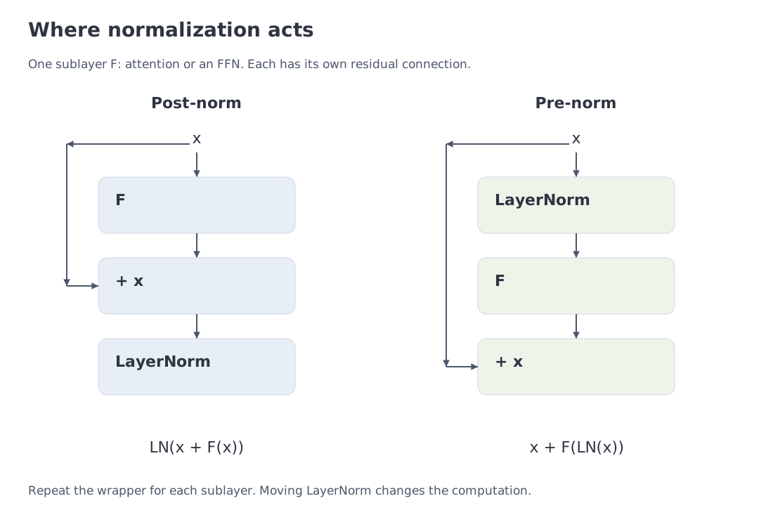 Each wrapper applies to one sublayer F, either attention or an FFN. The norm sits after residual addition on the left and inside the update branch on the right.
8.4. Dropout in the original recipe
Dropout randomly zeros some values during training and rescales the retained values; ordinary generation disables it. The original Transformer applies it to sublayer outputs before residual addition and to the sum of token and positional embeddings. We omit it from the equations above to keep the paths visible.
9. The encoder layer and encoder stack
One encoder layer performs two operations:
- bidirectional self-attention;
- a position-wise FFN.
Each has its own residual connection and LayerNorm. In post-norm notation,
The stack repeats the layer structure times, with separate learned parameters in each layer. The base paper uses . The final output is encoder memory:
Every source vector is now contextual: it can incorporate any unmasked source position.
9.1. When an encoder is useful
An encoder is useful when all input tokens are available, as in classification or document embeddings for search. Bidirectional attention lets a position read both left and right context. In a causal decoder-only model, even prompt positions can read only their own prefixes; the final prompt position can incorporate the entire prompt.
10. The decoder layer and cross-attention
The original decoder layer contains three sublayers:
- masked self-attention over the target prefix;
- cross-attention to encoder memory;
- an FFN.
In compact post-norm notation,
The second line takes queries from the decoder and keys/values from the encoder. The decoder can therefore select relevant source information for each target step.
10.1. Why the target is shifted
Suppose the correct target sequence is
I love models <EOS>
The decoder input is
<BOS> I love models
while the loss targets are
I love models <EOS>
Treat each word as one toy token here; a real tokenizer may split it further. <BOS> marks the start and <EOS> the end. The input is shifted by one token: the <BOS> position predicts “I,” the “I” position predicts “love,” and so on. The diagonal is allowed because the input token at a position is already part of the known prefix.
10.2. Linear projection and softmax
Each final position vector , or hidden state, is multiplied by . This produces one unnormalized score, called a logit, for each vocabulary item:
Probabilities are
Some models tie the output matrix to the input embedding matrix. Weight tying saves parameters and connects the token-reading and token-writing spaces, but it is not required by the Transformer architecture.
11. Training: teacher forcing and cross-entropy
Teacher forcing supplies the known target sequence shifted by one position. The model is scored using the negative log-likelihood (NLL) of the correct next token. Summing over a sequence gives
denotes the learned parameters, the target token, its prefix, and the source text in translation. Decoder-only modeling omits the separate source . We use natural logarithms, so NLL is measured in nats. For a target distribution concentrated on one correct token, this loss is also the cross-entropy between the target and the model distribution.
11.1. Why training is parallel
Although the probability factorization is autoregressive, every correct target token is already available in a training example. The complete shifted target is passed as one tensor, and the causal mask preserves validity. Positions are computed in parallel while each sees only its allowed prefix.
The distinction is fundamental:
- the distributional dependency is autoregressive;
- the training forward computation is parallel over positions.
11.2. A numerical NLL example
Suppose one position has vocabulary logits
Softmax gives
If the correct token has zero-based index 3, the position loss is
Cross-entropy, KL divergence, and the coding interpretation of NLL are derived in the companion course: Course Information Theory for ML, Module 3. The engineering reading here is sufficient: the loss charges the model according to the probability it assigned to the correct token.
11.3. Loss masks are not attention masks
Let for a prediction that should be scored and otherwise. The mean loss is
Padding targets are excluded. Training on prompt–answer pairs may also score only the answer. An attention mask controls access to information; a loss mask selects predictions for scoring. A token excluded from the loss may still be available as context.
12. Generation: the same forward pass in a different loop
During generation, the next target token is not provided. The algorithm is:
- pass the current prefix to the model;
- read logits at the final position;
- select the next token;
- append it to the prefix;
- repeat until
<EOS>or a length limit.
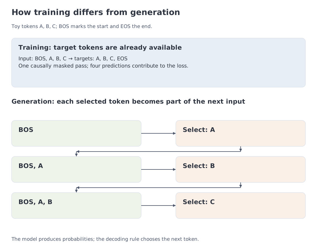 The same computation produces a next-token distribution. Training supplies known prefixes; generation extends a prefix with the model’s own choices.
12.1. Greedy selection, sampling, and decoding policy
The forward pass ends with one logit per vocabulary ID. Turning those scores into a token is a separate decision. Greedy decoding takes the largest score. Sampling draws from a probability distribution, so repeated runs can continue the same prefix differently.
A positive temperature changes that distribution:
At this is ordinary softmax. A temperature below one concentrates mass on higher logits; a temperature above one spreads it more evenly. Positive temperature preserves the ranking, so it does not change the greedy choice. The formula does not admit division by zero. An interface that uses temperature=0 to request greedy decoding is selecting a separate rule.
For logits , temperature one gives approximately . At temperature two the probabilities become . Greedy decoding still selects ID 0, while sampling is now more likely to pick one of the other IDs. Greater diversity alone says nothing about whether those alternatives solve the task better.
We can also restrict the candidate set . Top-k keeps the most probable IDs. Top-p, also called nucleus sampling, sorts candidates by probability and keeps the shortest prefix whose cumulative mass reaches . The candidate that crosses the threshold is included. Either filter requires renormalization before drawing a token:
Apply the filters separately at temperature one. Top-k with keeps IDs 0 and 1, yielding . With top-p at , those two IDs contribute only about 0.880797. Including ID 2 raises the retained mass to 0.967941, and renormalization gives . Top-k fixes a count; top-p lets the count adapt to the current distribution. See Holtzman et al., Section 3 for the definition and original motivation of nucleus sampling.
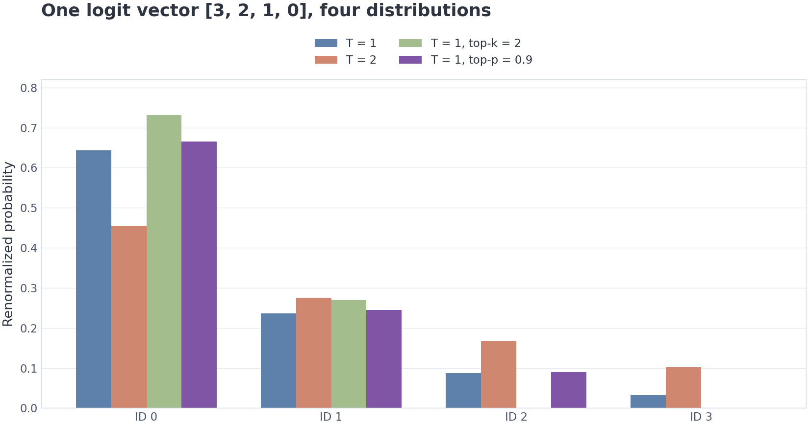 Every series starts from the same logits. The two filters are applied separately at temperature one; a zero-height bar marks an excluded ID.
The notebook implements exponentiation, sorting, cumulative mass, and renormalization explicitly. It resolves equal logits by ID. When filters are combined, its order is temperature, top-k, then top-p; the final threshold is measured within the retained top-k distribution. Record that order as part of the generation protocol. Module 11 will preserve a target sampling distribution, which includes these transformations rather than only the model's raw softmax.
12.1.1. Stopping the loop
After selection, the new token joins the prefix used by the next forward pass. An EOS token—end of sequence— terminates the sequence. Dialogue formats may instead define particular end-of-turn markers; Module 13 explains that contract. A separate cap limits the number of new tokens. Reaching the cap is a different stopping reason from the model emitting an end marker.
A filter can exclude EOS at one step, while the next step has a different logit vector. Neither greedy decoding nor sampling by itself guarantees that an end marker will arrive in time. The notebook checks EOS termination and length termination on prepared score traces. These traces isolate loop control; they do not evaluate a trained model's answer quality.
12.2. Why errors can accumulate
Training prefixes are correct. During generation, an early poor token becomes part of the next input. The model may enter prefix regions that were rare in training. This is one reason token-level loss and long-form generation quality are not identical quantities.
12.3. Why a KV cache works
In a causal stack, an old token’s representation depends only on its existing prefix. Appending a token therefore leaves old keys and values unchanged as long as weights, positions, and available context stay fixed and dropout is disabled. A KV cache stores those keys and values at each layer. A new token contributes one query row while the stored key/value sequence grows. Editing the prefix or renumbering positions requires reconsidering cache validity.
Module 10 develops KV-cache memory and request serving. For an optional connection to reinforcement learning, RL for LLM, Module 6, treats token selection as an action under a policy. That perspective is not needed for the computation here.
13. A minimal scaled dot-product attention implementation
Run the code blocks in §§13–14 in order. This teaching version exposes the calculation and its main input checks: finite floating-point tensors with nonempty axes on one device, and a Boolean mask broadcastable to the score shape. It computes in float32 or float64 and returns (output, weights). The notebook adds diagnostic fields and padding support.
from __future__ import annotations

import math
from typing import Literal

import torch
from torch import Tensor

def scaled_dot_product_attention(
    q: Tensor,
    k: Tensor,
    v: Tensor,
    allowed: Tensor | None = None,
    *,
    empty_row: Literal["error", "zero"] = "error",
) -> tuple[Tensor, Tensor]:
    """Educational attention with an explicit fully-masked-row policy.

    q: [..., T_q, d_k]
    k: [..., T_k, d_k]
    v: [..., T_k, d_v]
    allowed: broadcastable bool mask [..., T_q, T_k], True = allowed
    """
    if empty_row not in {"error", "zero"}:
        raise ValueError("empty_row must be 'error' or 'zero'")
    if min(q.ndim, k.ndim, v.ndim) < 2:
        raise ValueError("q, k and v must have at least two dimensions")
    if any(size <= 0 for t in (q, k, v) for size in t.shape):
        raise ValueError("q, k and v must have non-empty axes")
    if not all(t.is_floating_point() and torch.isfinite(t).all() for t in (q, k, v)):
        raise ValueError("q, k and v must be finite floating-point tensors")
    if not (q.device == k.device == v.device):
        raise ValueError("q, k and v must be on one device")
    if q.shape[-1] != k.shape[-1]:
        raise ValueError("q and k must share d_k")
    if k.shape[-2] != v.shape[-2]:
        raise ValueError("k and v must share T_k")

    dtype = torch.float64 if torch.float64 in {q.dtype, k.dtype, v.dtype} else torch.float32
    q, k, v = (t.to(dtype=dtype) for t in (q, k, v))
    batch_shape = torch.broadcast_shapes(q.shape[:-2], k.shape[:-2], v.shape[:-2])
    q, k, v = (t.expand(*batch_shape, *t.shape[-2:]) for t in (q, k, v))
    scores = (q @ k.transpose(-2, -1)) / math.sqrt(q.shape[-1])

    if not torch.isfinite(scores).all():
        raise FloatingPointError("attention scores overflowed")

    if allowed is None:
        allowed = torch.ones_like(scores, dtype=torch.bool)
    else:
        if allowed.dtype is not torch.bool:
            raise TypeError("allowed must be a bool mask")
        allowed = torch.broadcast_to(allowed.to(scores.device), scores.shape)

    empty = ~allowed.any(dim=-1)
    if empty_row == "error" and empty.any():
        raise ValueError("attention contains a fully masked row")

    masked_scores = scores.masked_fill(~allowed, float("-inf"))
    row_max = torch.where(
        (~empty)[..., None],
        masked_scores.max(dim=-1, keepdim=True).values,
        torch.zeros_like(masked_scores[..., :1]),
    )
    exponentials = torch.where(
        allowed,
        torch.exp(masked_scores - row_max),
        torch.zeros_like(masked_scores),
    )
    denominator = exponentials.sum(dim=-1, keepdim=True)
    denominator = torch.where(denominator > 0, denominator, torch.ones_like(denominator))
    weights = exponentials / denominator
    output = weights @ v
    if not torch.isfinite(output).all():
        raise FloatingPointError("attention output overflowed")
    return output, weights
A fully masked row is not a probability distribution: naive softmax([-inf, …, -inf]) produces NaN. The safe default is therefore an error. Enable the zero policy only explicitly—for example, for a padded query whose attention output should be zero.
13.1. A causal mask
def causal_allowed(
    t_q: int,
    t_k: int,
    *,
    query_offset: int = 0,
    device=None,
) -> Tensor:
    if any(type(n) is not int for n in (t_q, t_k, query_offset)):
        raise TypeError("lengths and offset must be integers")
    if min(t_q, t_k) <= 0 or query_offset < 0:
        raise ValueError("positive lengths and non-negative offset required")
    q_pos = query_offset + torch.arange(t_q, device=device)[:, None]
    k_pos = torch.arange(t_k, device=device)[None, :]
    return k_pos <= q_pos
For ordinary self-attention, and query_offset=0. During cached decoding, the new query may have local index zero but global position ; use query_offset=t, otherwise the mask incorrectly permits only the first key.
13.2. A minimal multi-head module
import torch.nn as nn

class MultiHeadSelfAttention(nn.Module):
    def __init__(self, d_model: int, n_heads: int) -> None:
        super().__init__()
        if any(type(n) is not int or n <= 0 for n in (d_model, n_heads)):
            raise ValueError("d_model and n_heads must be positive integers")
        if d_model % n_heads != 0:
            raise ValueError("d_model must be divisible by n_heads")
        self.d_model = d_model
        self.n_heads = n_heads
        self.d_head = d_model // n_heads
        self.qkv = nn.Linear(d_model, 3 * d_model, bias=False)
        self.out = nn.Linear(d_model, d_model, bias=False)

    def forward(self, x: Tensor, causal: bool = True) -> Tensor:
        b, t, _ = x.shape
        qkv = self.qkv(x)
        q, k, v = qkv.chunk(3, dim=-1)

        def split_heads(z: Tensor) -> Tensor:
            return z.view(b, t, self.n_heads, self.d_head).transpose(1, 2)

        q, k, v = map(split_heads, (q, k, v))
        allowed = None
        if causal:
            allowed = torch.ones(t, t, dtype=torch.bool, device=x.device).tril()
        y, _ = scaled_dot_product_attention(q, k, v, allowed)
        y = y.transpose(1, 2).contiguous().view(b, t, self.d_model)
        return self.out(y.to(dtype=x.dtype))
Once the explicit computation is clear, compare it with torch.nn.functional.scaled_dot_product_attention. The function selects an available implementation based on the device, dtype, and mask. Calling it does not guarantee FlashAttention or the absence of full intermediate matrices. The notebook compares outputs and gradients with dropout_p=0.0 set explicitly.
14. A minimal Transformer block
We now assemble a small decoder-only block with normalization before each sublayer. Its FFN uses GELU, the smooth nonlinearity , where is the standard normal cumulative distribution function. This teaching variant uses pre-norm and GELU; the 2017 architecture uses post-norm and ReLU.
class FeedForward(nn.Module):
    def __init__(self, d_model: int, d_ff: int) -> None:
        super().__init__()
        self.net = nn.Sequential(
            nn.Linear(d_model, d_ff),
            nn.GELU(),
            nn.Linear(d_ff, d_model),
        )

    def forward(self, x: Tensor) -> Tensor:
        return self.net(x)

class DecoderBlock(nn.Module):
    def __init__(self, d_model: int, n_heads: int, d_ff: int) -> None:
        super().__init__()
        self.ln1 = nn.LayerNorm(d_model)
        self.attn = MultiHeadSelfAttention(d_model, n_heads)
        self.ln2 = nn.LayerNorm(d_model)
        self.ffn = FeedForward(d_model, d_ff)

    def forward(self, x: Tensor) -> Tensor:
        x = x + self.attn(self.ln1(x), causal=True)
        x = x + self.ffn(self.ln2(x))
        return x
Read the graph in words:
ln1(x)normalizes every position;- causal self-attention mixes only the admissible prefix;
- its output is added to the original
x; - a second norm+FFN transforms every position;
- another residual connection preserves route and shape.
14.1. Causal invariance as a unit test
A strong mask test changes a future token and checks that earlier outputs do not change. For position ,
Keep weights fixed and use eval() so dropout cannot create unrelated differences. Compare floating-point outputs with torch.testing.assert_close. Include an unmasked control to show that the chosen example can actually expose future leakage.
15. A complete shape trace for a toy model
Let
- ;
- ;
- ;
- ;
- ;
- ;
- .
One decoder-only forward pass has the following shapes:
| Stage | Shape |
|---|---|
| token ids | |
| embedding + position | |
| packed QKV | |
| Q/K/V after splitting heads | |
| scores | |
| per-head attention output | |
| concatenation + | |
| FFN hidden state | |
| block output | |
| vocabulary logits |
This table is a practical debugger. Most first-implementation failures are not in the mathematics. They are in transpose, view, mask broadcasting, or the softmax axis.
15.1. Counting the main projection weights
Return now from the toy dimensions to the paper’s base configuration: , . For one layer, excluding biases, LayerNorm parameters, and embeddings:
- encoder self-attention: ;
- FFN: ;
- encoder layer: ;
- decoder layer: two attention sublayers plus the FFN = .
These counts are exact under the stated exclusions. A complete layer also has biases and normalization parameters; a complete model adds embeddings, the vocabulary projection, and multiple layers. The comparison explains the large FFN share: its two wide matrices contain twice as many weights as the four MHA projections.
16. The 2017 original and a modern LLM: what survived
The word “Transformer” can misleadingly suggest one fixed architecture. In practice it names a family.
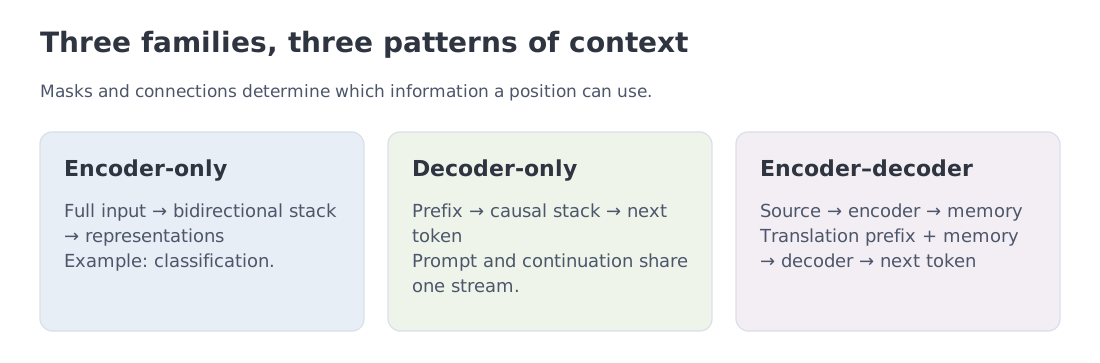 All three families use the same construction kit but differ in masks and information flow. Modern LLMs center the decoder-only branch, while encoders and cross-attention remain important for understanding the origin of the architecture and many multimodal systems.
Reference map. The replacement names below point to later chapters: positions in M4, attention variants in M5, norms and FFNs in M6, pretraining in M9, and execution in M10. They describe common choices rather than requirements for every LLM.
| Component | Original Transformer | Typical modern decoder-only LLM |
|---|---|---|
| architecture | encoder–decoder | decoder-only |
| attention | MHA | MHA, GQA, MQA, MLA, or a hybrid |
| position | sinusoidal absolute | usually RoPE and extensions |
| normalization order | post-norm | usually pre-norm |
| normalization | LayerNorm | often RMSNorm |
| FFN | ReLU MLP | often SwiGLU/gated MLP |
| task | seq2seq translation | next-token pretraining |
| inference | autoregressive decoder | autoregressive decoder + KV cache |
| efficiency | ordinary attention computation | FlashAttention, fused kernels, paging |
16.1. The stable core
Despite those replacements, the recognizable path remains:
- discrete tokens become vectors;
- positions and masks define sequence structure;
- attention routes information across positions;
- the FFN transforms each position nonlinearly;
- residual connections and normalization support a deep stack;
- a vocabulary head defines the next-token distribution.
This connects Module 2’s embeddings to the positional mechanisms in Module 4. The rest of the course asks how to scale, stabilize, train, serve, and extend it.
16.2. Why GPT is more than “a Transformer with the encoder removed”
Formally, a decoder-only stack removes the encoder and cross-attention. The more useful positive description is a stack of causal self-attention blocks trained on a next-token objective. Prompt and continuation occupy one token stream. The graph is not merely truncated; its dominant training and deployment regime is different.
17. Common confusions
17.1. “Attention stores knowledge”
The weights are computed afresh from the current input. Learned projection, FFN, and embedding matrices persist across requests. Keep those model parameters distinct from temporary mixing weights. The size of the FFN alone does not establish what fraction of the model’s knowledge it stores.
17.2. “A large attention weight proves causality”
A weight is a local mixture coefficient for one head and one layer. It omits residual paths, other heads, transformed values, FFNs, and later layers. It is a diagnostic signal, not a universal explanation.
17.3. “A causal mask makes computation sequential”
It makes the dependency causal. The training forward pass is still parallel over positions. The generation loop is sequential because future tokens do not yet exist.
17.4. “Self-attention is always square”
Scores have shape . Ordinary self-attention uses , but cross-attention and cached decoding may be rectangular.
17.5. “Heads split the input features before projection”
Each head projects from all input features. It is the projected result that is partitioned into heads, conventionally with width . Different heads can therefore use the same input coordinates.
17.6. “LayerNorm normalizes the batch”
LayerNorm normalizes features within one token position. BatchNorm uses statistics across examples; it is a different operation.
17.7. “Masking after softmax is equivalent”
Simply zeroing weights after softmax makes row sums smaller than one. Renormalization is possible but unnecessary and easy to destabilize. The canonical operation modifies logits before softmax.
17.8. “Post-norm and pre-norm differ only in the drawing”
Norm placement changes signal and gradient routes. The equation and the code must describe the same variant.
17.9. “Input embeddings and the output head must share weights”
Weight tying is common, not mandatory. Inspect the model configuration and implementation.
17.10. “The basic Transformer explains everything about modern LLMs”
It explains the computational skeleton. Data, optimization, scaling laws, post-training, retrieval, serving, multimodality, and evaluation are separate systems covered by the core course.
21. Reading route and sources
The following resources serve different purposes rather than duplicating one another.
- Primary source: Vaswani et al., “Attention Is All You Need”. Read the abstract, §3, Figure 1, §5, and the hyperparameter table before attempting the full training setup.
- Visual intuition: Jay Alammar, “The Illustrated Transformer”. A strong first pass through encoder–decoder flow and Q/K/V.
- Text next to code: Harvard NLP, “The Annotated Transformer” and its repository. Useful for matching the paper to an implementation.
- Geometric intuition: 3Blue1Brown, “Attention in transformers” and “Transformers, the tech behind LLMs”.
- Building a decoder-only model from scratch: Andrej Karpathy, “Let’s build GPT” and the Zero to Hero route. This is the GPT branch, not an exact encoder–decoder reproduction.
- A textbook with exercises: Dive into Deep Learning, Transformer chapter.
- Modern PyTorch API: the Scaled Dot Product Attention tutorial and function documentation.
- A compact self-attention implementation: Sebastian Raschka, “Understanding and Coding Self-Attention…”.
A useful route for a newcomer is: this lesson → Alammar → the notebook → Figure 1 and §3 of the paper → Karpathy or the Annotated Transformer. Experienced readers may need only the paper, VIZ 11, and the notebook tests.
22. Final cheat sheet and the next step
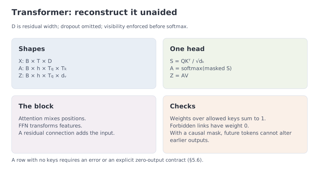 Four panels to reconstruct from memory: tensor shapes, one attention head, the role of each sublayer, and correctness checks.
The complete route is now compact:
- a tokenizer produces ids; embeddings and positions turn them into ;
- produces connection logits, a mask removes forbidden links, and softmax normalizes over keys;
- mixes values, heads are joined through ;
- the FFN transforms each position, while residual connections and normalization support a deep stack;
- the encoder reads the complete source; the decoder reads only its target prefix and, when present, encoder memory;
- teacher forcing trains all positions in parallel, while generation creates them sequentially;
- modern LLMs replace positional methods, norms, FFNs, head layouts, and kernels, but this computational skeleton remains recognizable.
Next: Module 4, positional representations, examines how the model represents token order and what happens when context grows beyond the lengths used in training.
Stable mathematical foundations. Modules 4–6 and 10 develop modern variants of these mechanisms. Cross-entropy/KL theory: Information Theory for ML, Module 3. The token model viewed as a policy: RL for LLM, Module 6.