Module 1. The Modern LLM Landscape
Modern LLMs · revision 2026.10.23 · release survey dated 11 October 2026
A release announcement gives you specifications, claims, and unanswered questions. This module turns them into a decision you can check. We will build a model passport, recording the model's properties and available evidence, and a system passport, recording how it is used and evaluated. Resource estimates will help us test those descriptions. The running example is an assistant that answers questions about internal documents and cites its sources.
You should have a broad idea of how neural networks learn from examples and how language models generate text from a prompt. You do not need to know Transformer internals. We will explain new terms when they become useful, then develop the mechanisms across the course: Module 2 introduces tokenization and embeddings, and Module 3 connects them to the Transformer computation. The calculations use algebra and powers of two; the exercises use Python functions and dictionaries.
Choose a route
| Pass | Read | What it enables |
|---|---|---|
| First: understand the task and its checks | Sections 1–2 → 4–6 → 8–12 → 15 → 19–22; E1, E5, and E6 | Explain the model's role, estimate weight storage, and distinguish an answer from its supporting evidence |
| Second: reproduce the estimates | The optional details in 5–6 and 8 → Section 7 → Sections 16–18; E2 and the full notebook | Interpret a configuration, reproduce parameter and resource estimates, and state their assumptions |
| Reference: examine a release | Section 3, Sections 13–14 and 23; projects E3–E4 | Separate artefact properties, provider claims, and unknowns |
On the first pass, skip only blocks labelled Second pass or Optional case. Read the remaining prose of the selected sections in order. Section 22 marks training compute separately as second-pass material. Architecture tables are an index to later explanations; you do not need to memorize their acronyms.
The notebook starts with three short, self-contained sections: an answer and its evidence, weight storage, and cost per accepted task. The later sections expose the detailed accounting and validation. Run all executes the required path in order without calling a model API.
1. Start with a decision
A document assistant is a program that finds information in a defined document collection and uses it to answer questions with citations. An employee might ask how long a report must be retained; the assistant locates the relevant policy and explains the requirement. That task spans retrieval, language generation, and checking that the cited passage supports the answer.
You could build it around a remote service, accessed through an API—an application programming interface—or run a model on your own hardware using downloadable weights, the numerical parameters learned during training. Either route offers models with different capabilities and costs. Some also let you control the amount of computation spent on a response. Availability and price per call are useful facts, but neither tells you whether the assistant will solve the task.
To compare the options, we need a more precise account of the model's role. A large language model (LLM) processes text as tokens, units that may represent words, word fragments, punctuation, or other pieces. In the usual autoregressive setup, the model scores the next token from the text available to it; the program selects a token, appends it, and repeats. Applying a trained model is called inference. This generation order is the course's main setting; Module 12 develops an alternative.
The model and the system therefore have different responsibilities. The model computes token scores. The system retrieves documents, prepares the input, supplies tools, and checks the result. The same weights can give different task outcomes in a bare chat interface and in a program with retrieval. Even a correct answer can cite a passage that does not support it. Section 12 makes this distinction concrete; Module 17 develops document retrieval, and Module 19 examines evaluation.
We will organize the comparison around six questions: how much memory the weights need, how much text the model can use, which data types it accepts and produces, how computation is allocated to an answer, which artefacts and usage rights are available, and how much an accepted result costs. Model properties and their evidence belong in the model passport. Runtime settings, measurements, and acceptance rules belong in the system passport.
Fill in both records as you read. Keep unpublished or unmeasured fields marked as unknown. Section 12 connects expenditure to accepted answers, and Section 15 examines the evidence behind comparisons. Product names will change; the method remains useful.
2. From a small calculation to an implementation you can read
The course asks you to understand models as well as compare them. We will revisit mechanisms in several forms: a short calculation, a controlled experiment, a passage of existing source code, and a small model assembled from the pieces. Each form has a different learning purpose. Running on physical hardware is common to all of them; it is not a certificate of operational readiness.
| Form of work | Question | Result to aim for |
|---|---|---|
| 1. Minimal implementation | How does the formula become a computation? | A short program with each essential step visible |
| 2. Practical notebook | Does the calculation remain meaningful on different inputs? | A reproducible experiment with shape, unit, and boundary checks |
| 3. Reading an open implementation | Where does the familiar mechanism appear in an existing model? | A comparison of the formula, configuration, and selected source code |
| 4. Integrated final project | How do the mechanisms work together? | A compact MiniLLM model that can be trained, modified, and tested |
The minimal version makes the idea inspectable. A practical notebook adds enough discipline to reproduce and change the experiment: a weight-storage calculation should reject a negative parameter count or zero bits per weight. Input checks turn the formula's assumptions into an explicit part of the program.
Reading an open implementation means locating operations such as a matrix projection, activation, or expert selection and relating them to the teaching version. The same repository may also contain specialized kernels and code for multiple devices. Developing those components is outside this course. We use resource and communication estimates to understand constraints; we do not teach the implementation of distributed training, kernel development, or the operational work required to deliver a production service.
A few model families recur as reading examples. gpt-oss provides configurations that can be compared with open implementation code. DeepSeek supplies detailed architecture reports, and OLMo exposes more of the training process. Inkling and Tinker illustrate downloadable weights combined with a managed adaptation service. Section 14 introduces their technical signatures after the comparison questions have acquired meaning.
The fourth form of work is the final project. It brings the studied mechanisms together in MiniLLM, a small trainable model with saved state, configurable variants, and executable checks. You can investigate how a change affects its behaviour at an accessible scale. Turning that reference implementation into a reliable service for users would require a separate engineering project and further study.
How large is MiniLLM? The same implementation supports three sizes, S, M, and L, with two architecture choices at each size. A dense model sends every token through the same computational blocks. A Mixture of Experts (MoE) model replaces some of those blocks with collections of subnetworks called experts, selecting only a few experts for each token. It therefore has two useful parameter counts: all the parameters it stores, and the active parameters attributed to processing one token. Module 7 develops expert selection; here the distinction gives us a first view of the project's scale.
The table also shows the dimensions behind each size. Layers are repeated processing stages; width is the number of components in a token's internal vector. Vocabulary size counts the distinct tokens, while context is the maximum sequence length configured for the profile, in tokens. Modules 2–5 explain these dimensions in detail. Parameter counts below are in millions, rounded to two decimal places.
| Size | Layers × width | Vocabulary | Context | Dense: parameters, million | MoE: total, million | MoE: active, million |
|---|---|---|---|---|---|---|
| S | 6 × 256 | 8 192 | 512 | 6.33 | 20.36 | 6.59 |
| M | 8 × 512 | 16 384 | 1 024 | 30.94 | 174.88 | 30.37 |
| L | 20 × 2 048 | 32 768 | 2 048 | 1 020.35 | 10 020.54 | 1 055.21 |
Source: the six MiniLLMConfig.profile() presets in the capstone implementation. Each dense/MoE pair shares its depth, width, vocabulary, and context. The capstone's active-count convention includes shared matrices in full, including vocabulary matrices, and only the selected experts from each routed bank. For a dense model, this convention gives the total parameter count. Section 6 explains the limits of this accounting.
S supports short experiments and checks of the complete workflow; M provides a larger setting for learning experiments. L is an optional move into the billion-parameter range: about 1.02 billion parameters for dense and 10.02 billion for MoE. Required exercises reduce the configurations further. Training L needs a separate compute budget, and L-MoE serves primarily as a resource-accounting example. Similar active counts do not imply equal speed, and the MoE model still needs storage for all its weights.
These profiles let us study architectural choices through a complete training workflow at several scales. The quality of the resulting text depends on training data, training budget, and evaluation on held-out tasks; model dimensions alone cannot establish what the model can do. The capstone guide explains how to choose a manageable run.
Across all four forms of work, we need to know where a model's weights are stored and how its design is documented. A saved set of weights is a checkpoint. A config.json file usually specifies architectural dimensions and choices, while a model card describes training, intended use, and limitations. The checkpoint holds parameter values; the configuration supplies dimensions; the code defines operations; and the card adds provenance and usage conditions. We will use these complementary sources together to build a verifiable model passport.
3. Nine years in fifteen minutes: 2017 → 2026
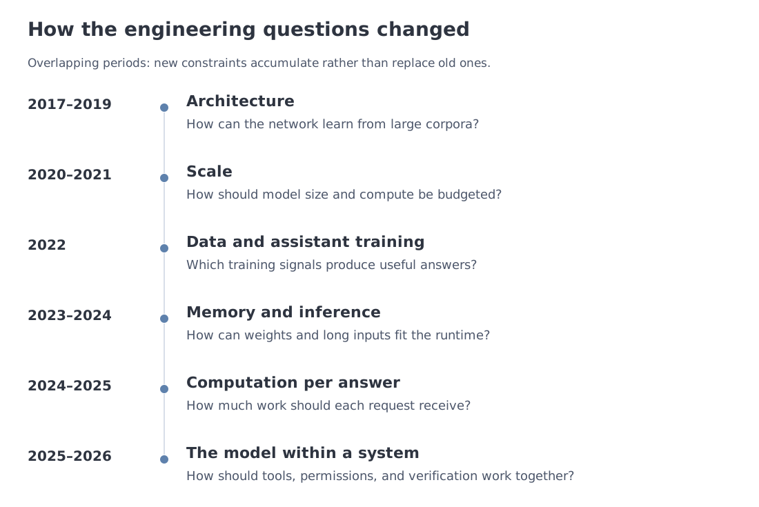 Six eras: architecture, scale, data, inference, post-training, and system orchestration. Release names stay in the table so the timeline remains readable.
A useful history of LLMs is not a parade of release names. It is a history of changing bottlenecks.
2017–2019: architecture. The Transformer enabled parallel training across sequence positions. GPT and BERT established pretraining followed by adaptation as a general approach. The immediate challenge was to build an architecture that could learn from large corpora.
2020–2021: scale and in-context learning. GPT-3 demonstrated broad task adaptation through instructions and examples without weight updates. Scaling laws helped turn model size and training compute into quantities that could be budgeted.
2022: data and alignment. Chinchilla showed why parameter count and training-token count must be chosen together. InstructGPT and ChatGPT highlighted the roles of supervised fine-tuning, preferences, reward, and the user interface in turning a language model into an assistant.
2023–2024: open weights, MoE, and long context. Llama, Mixtral, and DeepSeek made architecture comparisons widely accessible. GQA, MLA, sparse experts, efficient attention kernels, and longer contexts brought memory and inference bandwidth to the centre of the discussion.
2024–2025: reasoning and test-time computation. Reasoning models, reinforcement learning with verifiable rewards (RLVR), verification, distillation, and multi-token prediction expanded the ways compute could be allocated. The budget for an individual request became an explicit design choice.
2025–2026: systems. A checkpoint remains the computational core, but tools, memory, code execution, subagents, permissions, sampling, and the evaluation environment increasingly determine the result. These eras overlap: a new constraint adds to the earlier ones rather than replacing them.
A dated snapshot makes the last transition concrete without turning the history section into a news feed.
| Change | Examples as of 11 October 2026 | Passport question |
|---|---|---|
| Several cost and capability tiers | GPT-6 Astra / Sol / Luna, GPT-6.1 Sol; Claude Opus / Sonnet / Haiku 5.5 | Which version, effort, rate, and request limits apply? |
| Long-running agent tasks | Gemini 3.8 Flash, Grok 4.7 | Which tools, time limits, attempts, and acceptance criteria were used? |
| Staged availability | Gemini 4 Argon: announced, with restricted Fairwind access | Can this workload actually use the product? |
| New open architectures | Qwen3.8-2.4T-A95B; DeepSeek-V4.1-Flash | Which artefacts and licences exist, and does active count differ between prefill and decode? |
| The model operates inside a system | tools, persistent memory, multiple agents | How are permissions, coordination, verification, and total cost controlled? |
Sections 13–14 and 23 provide dates and primary sources for this snapshot.
The stable lesson is not the identity of a temporary leader. It is that each generation turns a formerly hidden cost into an explicit field in the passport.
4. Compare mechanisms before names
Begin inside the network. Attention combines information across context positions. A feed-forward network (FFN) transforms the vector at an individual position. Module 3 puts these operations together into a basic Transformer; Modules 5–7 examine their variants.
Three architecture questions are enough for this overview. Does each token use the same weight bank, or select part of a larger one? Does it consult the full available history, a local window, or a compressed state? What representations enter and leave the network? The first question leads to dense models and experts in Section 6. The second leads to context memory in Section 8.
An open model's config.json records some of the answers through dimensions, layer counts, and attention or expert settings. The implementation determines the actual computation. A family name cannot substitute for this evidence.
Architecture also leaves training history unspecified. Pretraining learns weights from a large corpus. Supervised fine-tuning (SFT) uses examples of desired responses. Reinforcement learning (RL) updates the model using signals about the quality of outcomes. Different data and adaptation can produce different behaviour at identical dimensions, so the passport needs training evidence and evaluation as well as a configuration.
5. Two passports: model and system
The model passport describes the computational core. The system passport records how it is used. A retrieval tool, for example, provides access to documents; it does not establish that an answer's citations are checked. That is a separate system rule.
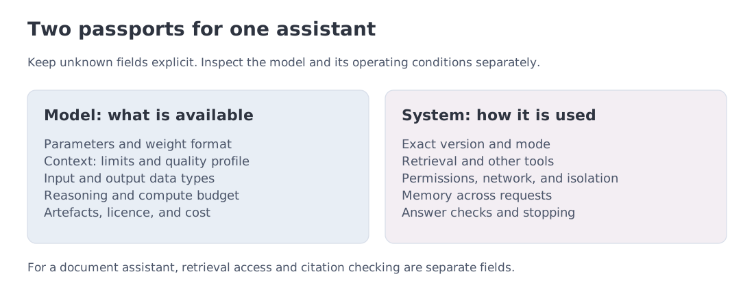 The model computes. The surrounding system supplies evidence and tools, controls actions, and checks the result.
A model property and a workload result have different evidence requirements. Configuration and code can establish a parameter count. Cost per accepted answer and long-context quality require a task, settings, and an acceptance rule. The model passport may link to those measurements, but the system passport records their conditions. A result from one workload must remain attached to that workload.
For the assistant in Section 1, the relevant question is whether it can find the applicable retention policy and support its answer from that policy. Parameter count does not establish either outcome. The system record must therefore specify the document collection and the acceptance check.
5.1. Record the model
| Field | Question for the document assistant | Evidence |
|---|---|---|
| Parameters | How many weights are stored and how many participate per token? | Configuration, code, card; §6–7 |
| Context | How much material is accepted, and at what length do answers remain useful? | Documentation and workload evaluation; §8 |
| Inputs and outputs | Must it read page images, or only text? | Model card and request format; §9 |
| Reasoning | Can difficult questions receive more computation? | Request controls and measurements; §10 |
| Access | Are weights and the required usage rights available? | Repository, licence, service terms; §11 |
| Economics | What do accepted answers cost, and how long do they take? | Rates and measured runs; §12 |
5.2. Record the system
| Field | What it establishes |
|---|---|
| Model version and mode | The exact variant under evaluation |
| Retrieval and other tools | The evidence and actions available to the assistant |
| Permissions, network, isolation | Which documents, files, and services can be affected |
| Memory across requests | What persists and who can access it |
| Evaluation protocol | Questions, budgets, and answer acceptance rules |
| Monitoring and stopping | How errors are detected and execution is ended |
The program coordinating model and tool calls is often called an agent harness. Here an agent is a system that can select and carry out a sequence of actions. Module 18 develops its design. For now, record the actions it is permitted to take.
5.3. First resource estimates
Let count all model parameters and count the parameters on one token's active path. An active count needs an explicit accounting convention (§6). In model sizes, B and T mean and parameters.
Weights are numbers, so their storage cost depends on the numerical format. BF16 uses 16 bits, or two bytes, per value. Quantization reduces that precision; effective storage must also include any scales and other format overhead.
For effective precision of bits per parameter,
A coarse estimate of weight-matrix arithmetic during generation is
The factor of two counts one multiplication and one addition per participating matrix weight. It estimates arithmetic, not elapsed time.
It excludes context-dependent attention, routing, normalization, sampling, communication, and poor hardware utilization.
Second pass: training compute
Training uses a different approximation,
whose assumptions are developed in Module 9.
Here is the parameter count under the chosen convention and the number of training tokens. This approximation includes forward and backward matrix operations.
Generating another token requires reading weights and retained context state. Moving these data can dominate runtime even when the device has a high arithmetic throughput. Modules 10–11 examine that cost.
Units matter. Vendors often quote file sizes and bandwidth in decimal GB/TB; accelerator memory is easier to read in binary GiB/TiB. FLOP counts operations, while FLOP/s is a rate. The course keeps those systems explicit.
6. Axis I up close: dense and MoE
In a dense Transformer, every token uses the same feed-forward blocks. In a Mixture of Experts (MoE) layer, a learned router selects a few experts from a larger bank. Selecting the highest-scoring experts is called top-k routing. Some designs also include a shared expert used by every token. The design therefore grows stored parameter capacity faster than the expert computation used by one token.
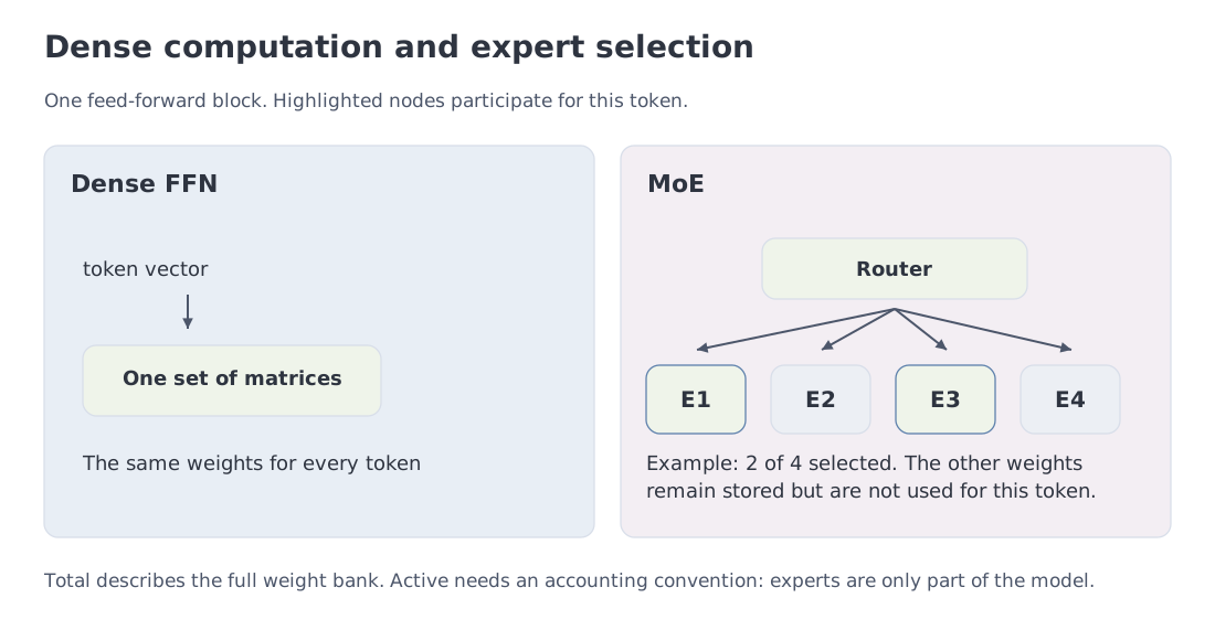 A dense FFN uses one set of weights. In this toy MoE, the router selects two of four experts; shared experts are omitted to keep the mechanism visible.
This is why MoE cards often report two sizes:
- total parameters: the full bank that the system must store and make available;
- active parameters: a declared or reconstructed convention for the path used by one token.
Second pass: active-count conventions and expert geometry
The active count depends on how operations are charged. An input embedding maps an ID to a vector; the output projection maps a model vector to scores for all next-token IDs. Module 2 develops both operations. Some cards include the full vocabulary projection, others report only the Transformer core; an input embedding may be charged as a row lookup rather than a full active matrix. A precise passport names the convention.
The open gpt-oss implementation makes the issue concrete. Counting visible matrices, biases, and learned attention sinks gives, for gpt-oss-120b,
under the course’s compute-oriented convention: the full output projection is included, while the indexed input embedding lookup is not charged as a full GEMM. The card rounds those values to 117B and 5.1B. Both are useful; they answer different questions.
MoE geometries vary widely.
| Model | Total / active | Routed experts / top-k | Shared path | Evidence |
|---|---|---|---|---|
| Llama 4 Scout | about 109B / 17B | 16 / 1 | yes | model card and config |
| gpt-oss-120b | 117B / 5.1B | 128 / 4 | no | official code and model card |
| DeepSeek-V4 Pro | 1.6T / 49B | reported in technical material | yes | technical report |
| Qwen3.8-2.4T-A95B | 2.4T / 95B | 512 / 10 | 1 | official config, checked 11 October |
| Inkling | 975B / 41B | 256 / 6 | 2 | official model card |
| Kimi K3 | 2.8T / 104B | 896 / 16 | 2 | official report/model summary |
| Nemotron 3 Ultra | 550B / 55B | LatentMoE | report-specific | official report |
Large experts with a small top-k reduce routing combinations but make every selected expert expensive. Fine-grained banks offer more combinations and lower active fractions, at the cost of load balancing, all-to-all traffic, and harder placement. Neither total/active nor expert count predicts quality on its own.
The practical reading rule is simple: in 1.6T / 49B, the first number says what the system must make available; the second gives a first estimate of weight work per token. The next step is to inspect the counting convention and implementation.
A phase-dependent example. Active count can depend on the execution phase. The DeepSeek-V4.1-Flash card reports 8B active parameters while processing the input (prefill) and 16B while generating subsequent tokens (decode). A passport may therefore need two active-count fields. Also check whether the reported total includes conditional memory and auxiliary components before comparing it with another model's total.
7. Worked comparison: gpt-oss-120b and Llama 4 Scout
These models have similar total parameter scale but make very different product and architecture choices.
The mechanism names in the table are reference labels for a second pass. The calculations use parameter counts, storage formats, and retained-state dimensions. Prefill processes the supplied input; decode adds new tokens sequentially.
| Passport field | gpt-oss-120b | Llama 4 Scout |
|---|---|---|
| Total / active | 117B / 5.1B; course reconstruction 116.829B / 5.133B | about 109B / 17B |
| MoE | 128 routed, top-4 | 16 experts, top-1 plus shared path |
| Attention | GQA 64/8; alternating full and 128-token sliding layers; learned sink per head | RoPE/NoPE hybrid, chunked attention, early-fusion multimodality |
| Context | 128K | up to 10M in the stated Scout mode |
| Distribution | MXFP4 expert weights; Apache 2.0 | BF16 and quantized paths; Llama Community License |
| I/O | text → text | text/image → text |
7.1. Weight artefact
For the teaching MXFP4 estimate, 32 four-bit weights share an eight-bit scale: bits per weight. Applying that rate uniformly to 117B parameters gives
The official source-weight index is 65,248,815,744 bytes, about 60.77 GiB. The difference is the lesson: a format name does not fully determine checkpoint size. Tensor precision is heterogeneous, and scales, metadata, and packing also occupy space.
7.2. Active arithmetic
Using the rounded card values,
for gpt-oss and
for Scout. This is not a promise of a threefold latency gap. Attention layout, expert placement, precision, kernels, and hardware are different.
7.3. Context state
A KV cache retains keys and values: computed vectors through which attention consults earlier positions. Full attention retains the available history; a sliding window needs only recent positions. Section 8 derives the general formula. For this example, use 8 key/value heads, 64 coordinates per head, and 2 bytes per coordinate (BF16).
An all-full equivalent for gpt-oss would cost 72 KiB of KV state per token across 36 layers, or 9 GiB at exactly 131,072 tokens. The actual schedule alternates 18 full-attention and 18 sliding-window layers; the Module 5 teaching calculation gives about
for one request, excluding metadata and workspaces and assuming the runtime retains only 128 positions in each local layer. A single sliding_window field is not enough—the layer schedule matters.
Scout advertises a much longer nominal context, but a serious passport asks three separate questions: will the runtime accept that length, does quality remain useful throughout it, and what memory/time does the chosen implementation require? “10M” begins the analysis; it does not finish it.
8. Axis II: context means length, quality, and cost
Context-window numbers look simple—128K, 1M, 10M—but encode at least three claims.
- Accepted length: the runtime and positional scheme permit the request.
- Quality at a given length: the model can retrieve and use the required information, tested for a particular task and evidence position.
- Economic length: the request meets memory, time, and cost limits. Two useful timings are time to first token (TTFT) and inter-token latency (ITL), the interval between subsequent output tokens.
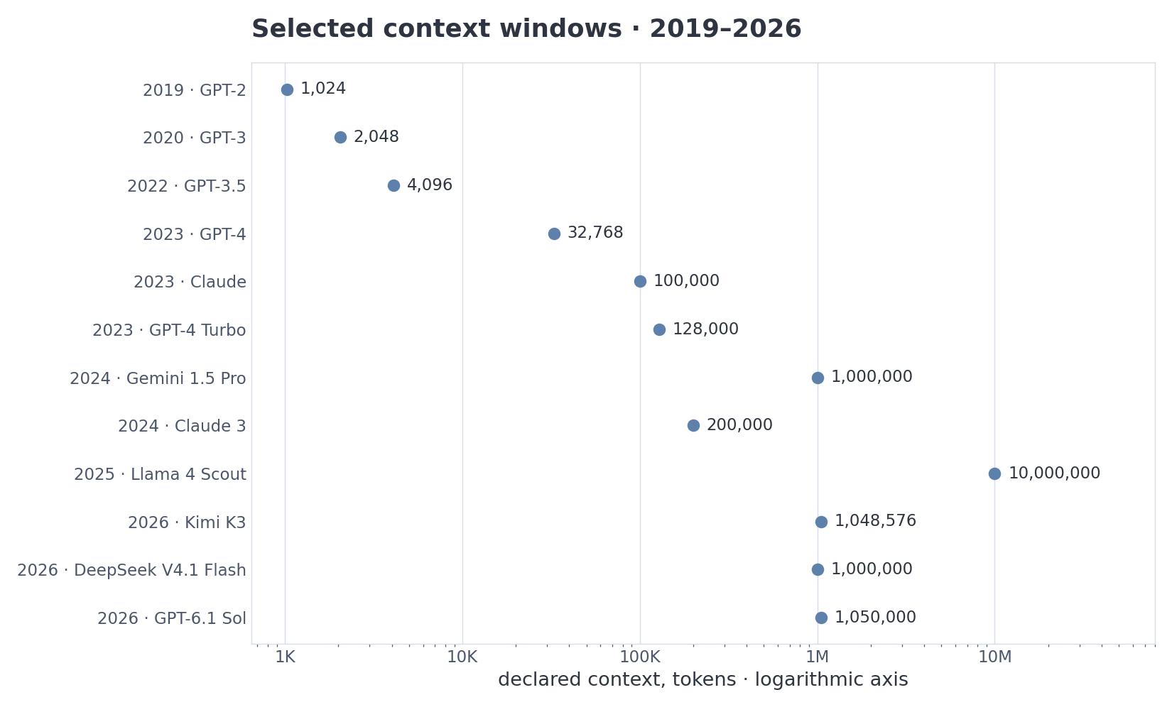 Selected declared context windows, 2019–2026. A logarithmic axis shows the range of advertised capacities; the points say nothing about answer quality, latency, or cost.
Second pass: the memory cost of context
Attention reads earlier positions through key and value vectors retained in a KV cache. Multiple attention heads can perform these operations in parallel. Grouped-Query Attention (GQA) shares keys and values across groups of query heads, so storage depends on the KV-head count. For a conventional cache, bytes per token across all cached layers are
Here counts cached layers, is the number of KV heads, is the head dimension, and is bytes per cache element. The weight-storage formula uses bits per parameter instead. For uniform full attention, multiply by sequence length to obtain per-request cache storage; hybrids and recurrent models need their own state calculation.
The leading factor of two counts keys and values separately. With , , , and , the cache uses 327,680 bytes per token: 305.18 GiB for exactly one million positions in one request. Compressed representations, local attention, recurrence, and cache quantization change this calculation (Modules 5, 8, and 10). Paged allocation reduces wasted allocated space; it does not itself shrink the stored vectors.
Needle-in-a-Haystack tests retrieval of a fact hidden in a long text. RULER combines several long-context task types; workload-specific tests expose further failure modes. A product still needs its own slice, recorded more like this:
The following is a hypothetical evaluation plan, not a measurement of a particular model. The 200,000 figure counts input tokens in one request, not documents.
Documented limit: 1,000,000 tokens; verify the combined input/output allowance
Test input: 200,000 tokens per request, documents from the teaching collection
Tasks: 100 questions with reference answers and supporting passages prepared in advance
Evidence positions: beginning, middle, end; repeat the same questions at each position
Acceptance: at least 90/100 correct, supported answers in each positional variant
Time to first token and memory: not yet measured
Retrieval-augmented generation (RAG) selects relevant documents before passing them to the model. Retrieval narrows the evidence; a long context lets the model compare the selected passages. Prompt caching separately reuses computation for repeated request prefixes. Our assistant may benefit from all three, but each needs a workload-specific check.
Working context is better described by a quality profile than by one universal length. The retention-period question may succeed near the beginning of a document and fail in the middle. A question requiring evidence from several distant passages imposes a different demand. Record the task, length, evidence positions, and acceptance rule. Module 19 develops the comparison and its uncertainty.
For the document assistant, separate the input and output limits from the conditions under which answer quality was tested. “Working” always refers to those conditions. For example, Google's 30 September Gemini 4 Argon announcement specifies a 1M-token output limit. That is not evidence of a 1M-token input window. The announcement also describes a restricted rollout.
9. Axis III: modalities are directional
So far, we have assumed that the assistant receives documents as text. Suppose a policy instead arrives as a photograph, with the retention period printed in a table. Before choosing a model, decide how that page will become usable evidence: through a separate text-recognition program or through the model's own visual path. The choice changes both the error sources and the resource budget.
A modality is a type of data, such as text, images, audio, or video. A multimodal passport needs to specify which types enter and which can be generated. A model may accept images but generate only text; produce speech without processing video; or fuse modalities at very different points in the network.
| Field | Example |
|---|---|
| Input | text + image + audio |
| Output | text only |
| Visual path | image encoder → dimension-matching connector → language model |
| Temporal order | how video frames and audio segments carry position information |
| Streaming | partial speech output supported or not |
| Limits | image count, audio duration, video FPS, visual-token cost |
An encoder converts the original signal to vectors; a connector makes them suitable for the language model. Each modality introduces a budget. Images become visual-token sequences, video adds a temporal axis, and streaming speech requires the system to coordinate input and output rates. Module 16 follows this path from image patches to omni systems and shows why one user interface need not imply one internal representation.
10. Axis IV: who controls the reasoning budget?
Finding one explicit retention period may require little more than reading the right sentence. Reconciling several instructions or checking an exception takes a different kind of work. That leads to a resource question: how much computation should the system spend before answering, and how will we determine whether it helped?
A model may spend different amounts of computation preparing an answer. The useful questions are who chooses that budget and which limits the interface actually enforces.
| Mode | Who selects the budget? | Product consequence |
|---|---|---|
| Instant | fixed or small internal budget | small reasoning budget; latency still needs measurement |
| Configurable effort | caller | explicit cost/quality trade-off |
| Adaptive thinking | model or controller | automatic allocation within configured limits |
| Separate high-compute mode | user selects another mode/model | more computation; task quality must still be evaluated |
| Multi-agent orchestration | external harness allocates work | parallel trajectories plus merge cost |
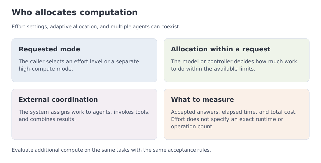 Reasoning modes differ not only in quality but in who controls test-time computation: caller, model, or external orchestration layer.
The modes above can be combined: a caller sets limits, then a controller allocates computation within them. A chain of thought is a sequence of intermediate reasoning steps; its visible length alone cannot measure reasoning capability. Some systems hide internal traces, others expose a separate channel, and still others spend the budget on tools or subagents. The passport should record effort settings, maximum output, tool access during reasoning, whether multi-agent is a separate system mode, and which safeguards apply.
Modules 13–15 explain instruction tuning, learning from preferences and verifiable rewards, transferring behaviour between models, and spending more computation while solving a task. The key lesson here is that the same model name at two effort or harness settings may denote two different evaluation objects.
An effort setting usually requests a mode; it does not promise an exact operation count, token count, or runtime. Caller-selected effort can coexist with adaptive allocation. More computation can also produce unnecessary edits or exhaust a time limit. For the document assistant, compare modes on the same questions, with fixed acceptance criteria and explicit time and spending limits. Module 15 develops this trade-off.
11. Axis V: access, licensing, and practical openness
Openness is better represented as a set of independent questions than as one line from closed to open.
| Question | Possible answers |
|---|---|
| Are weights downloadable? | no / gated / public |
| May a derivative be used commercially? | permissive / custom conditions / prohibited |
| Is inference code available? | snippet / framework integration / custom kernels |
| Is the training route available? | no / partial / code + data + logs |
| Can trained weights or an adapter—a smaller set of added parameters—be exported? | platform-dependent |
| Where can the model run? | local / partner API / hyperscaler / provider only |
| Can access change legally? | licence, export controls, regional restrictions |
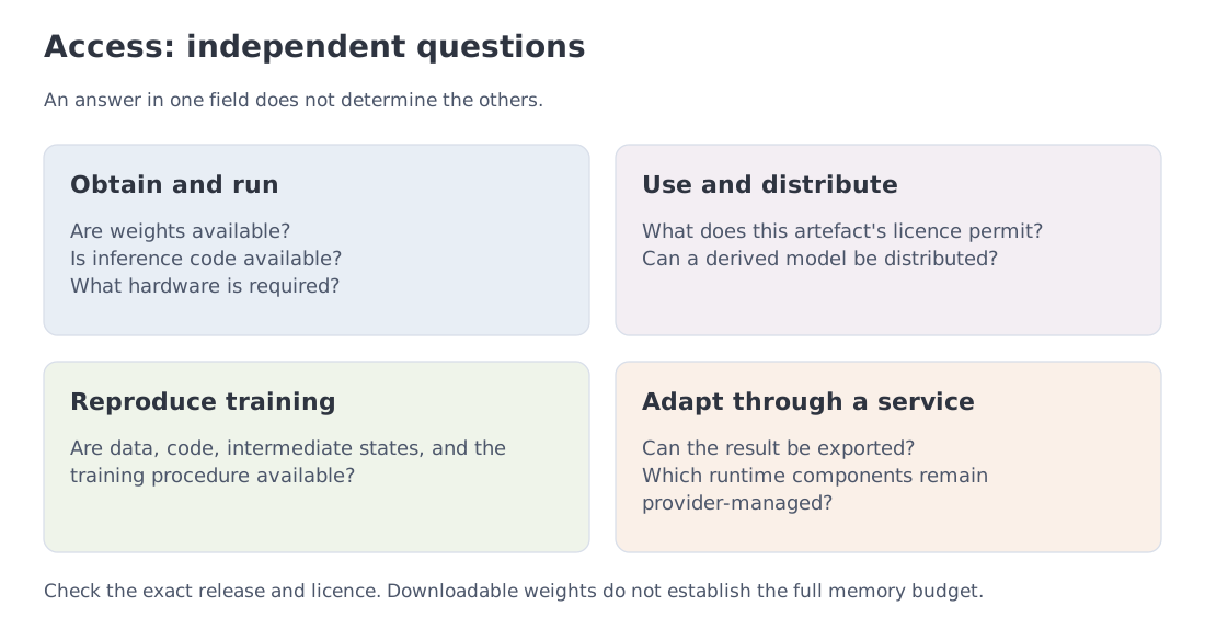 Weights, licence, code, data, and managed adaptation are separate coordinates.
Inkling and Tinker illustrate the distinction. Inkling publishes full model weights under Apache 2.0, while large-scale adaptation is also offered through a managed training API. A user can own the base artefact and the resulting adaptation without owning the entire distributed runtime.
Open weights do not imply easy deployment. Kimi K3 exposes a huge 2.8T-parameter bank; even a low-precision representation has a substantial weight payload. The device count depends on precision, usable memory per device, and the additional runtime state. gpt-oss-120b, by contrast, was packaged for the one-80-GB-GPU class. Licence and hardware footprint must be read together.
Self-hosting moves rather than removes the security burden. It grants control over data and runtime while transferring responsibility for the supply chain, sandbox, secrets, monitoring, and updates. Module 18 makes those responsibilities explicit.
Check the specific release, not just the family. Qwen3.8-27B is labelled Apache 2.0, whereas Qwen3.8-2.4T-A95B uses the custom qwen3.8-max licence. Sharing a family name does not establish identical usage rights.
12. Axis VI: from token prices to accepted answers
Token prices describe model calls; our decision concerns completed tasks. For the assistant in Section 1, completion means a correct answer supported by its source. An explicit acceptance rule connects these two units of comparison.
Consider an acceptance check using two fictional documents. They come from the independent teaching fixture document-assistant-v1, embedded in the notebook.
| Document | Passage |
|---|---|
| A — Experiment logs | “Keep an experiment log for 30 days after the experiment ends.” |
| B — Temporary exports | “Delete a temporary export 7 days after it is created.” |
The question is “How many days must an experiment log be kept after the experiment ends?” Consider three responses. “30 days, according to A” answers the question and cites supporting evidence. “7 days, according to A” gives the wrong period despite naming a real source. “30 days, according to B” gives the right number but cites a passage about something else. Answer correctness and source support are distinct checks. A link that opens successfully establishes neither on its own.
To prepare an answer, the program selects material relevant to the question and passes it to the language model along with instructions. The generated response then has to meet an acceptance rule. A person or a small program with a prepared reference can check this tightly bounded example. Checking arbitrary claims against arbitrary documents is a much harder task: Module 17 develops retrieval and source handling, while Module 19 examines how to evaluate the result.
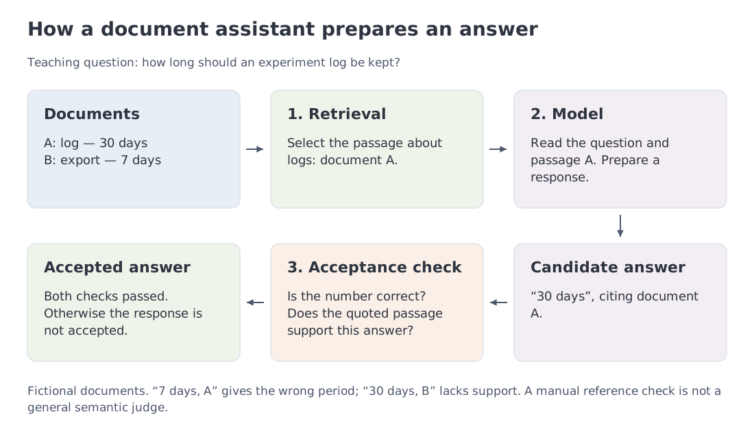 Retrieval selects evidence, the model prepares a response, and a separate check determines acceptance. A real citation may still fail to support an answer. Documents A and B are fictional teaching inputs.
All three calls could incur a charge, while only the first response would be accepted. We can now define the unit used in the cost comparison.
Start with the API bill: ordinary and cached input, output and billable reasoning tokens, retrieval, tools, execution environments, retries, and subagents. Then measure time to first token (TTFT), inter-token latency (ITL), end-to-end task time, and throughput at the required service-level objective (SLO). Context length, caching, and batch processing can change the applicable rates.
Set acceptance rules before comparing systems. A held-out set contains questions whose answers have not been used to select system settings. Repeatedly tuning on its errors makes it part of development; a final check then needs fresh questions. Module 19 develops this separation.
For task , let include every billed attempt and tool call. Let be 1 if the result meets a predefined acceptance criterion and 0 otherwise. On a fixed set of tasks,
Failed attempts still incur costs in the numerator. With no accepted tasks, the ratio is undefined. This is a measurement on a particular dataset, not a prediction for a retry-until-success policy.
Worked example. Evaluate two systems on the same 100 held-out questions. An accepted answer must be correct and supported by its citations. The prices and outcomes below are fictional teaching inputs, not current provider rates. Token totals include all attempts; there are no cache or batch discounts.
| Quantity over the entire run | System A | System B |
|---|---|---|
| Input / output, million tokens | 1 / 1 | 0.2 / 0.2 |
| Input / output price, USD per 1M | 1 / 2 | 2 / 10 |
| Tools, USD | 0.60 | 0.40 |
| Accepted tasks out of 100 | 60 | 80 |
| Total spend, USD | 3.60 | 2.80 |
| Spend per accepted task, USD | 0.060 | 0.035 |
A costs USD, or USD per accepted task. B costs USD, or USD per accepted task. B's higher token prices are offset by lower token consumption and more accepted answers. If the teaching requirement is at least 80 accepted tasks, only B passes. We have not measured latency, included human review or infrastructure, or established generalization beyond these questions. Module 19 addresses uncertainty and evaluation design.
For self-hosting, begin with
Then add KV or recurrent state, temporary buffers, kernel workspaces, concurrent requests, and redundancy. Compare an API with a hosted deployment under the same workload, including hardware utilization and operating costs. Irregular demand often suits an API; sustained volume, data-location requirements, or substantial customization can justify self-hosting. Modules 10, 11 develop the full cost model.
13. Dated reference: APIs and product availability
This snapshot records the primary-source evidence available on 11 October 2026. It selects families that illustrate passport questions; it is neither an exhaustive catalogue nor a ranking. Announcement, API access, and downloadable weights are separate events.
| Family | Confirmed update | Availability and engineering consequence |
|---|---|---|
| OpenAI | GPT-6 Astra on 3 September; GPT-6 Sol / Luna on 22 September; GPT-6.1 Sol on 29 September | The API changelog adds ultrafast for GPT-6.1 Sol on 8 October. A serving tier and its price do not disclose a new architecture |
| Anthropic | Opus 5.5, 22 September; Sonnet 5.5, 28 September; Haiku 5.5, 7 October | Record tier and effort. Sonnet's cache-read price changed on 7 October, so a pricing snapshot needs its own date |
| Google DeepMind | Gemini 3.8 Flash / Flash Cyber, 2 September; Gemini 4 Argon, 30 September | Flash is available through the Gemini API. Cyber and the announced Argon rollout use restricted Fairwind access; Argon's announcement does not establish general API availability |
| SpaceXSI | Grok 4.7, 21 September | Product and API access; no published architecture or weights. Record system tools and request settings separately |
| Qwen | Qwen3.8-Max and released Qwen3.8-2.4T-A95B weights | The weight card distinguishes the text checkpoint from the API product's additional features. Check the contract of each artefact separately |
| DeepSeek | V4 Pro GA on 13 August; V4.1 Flash on 10 September | The revised API changelog retains V4 Pro and routes old V4 Flash names to V4.1 Flash. An unchanged request string can now select a different model |
For a concrete contract, GPT-6.1 Sol documents a 1,050,000-token context window and a 128,000-token maximum output. These limits must not be added as independent input and output allowances. Reproducing a comparison also requires effort, API version, tools, and the applicable pricing conditions.
Some fields remain unknown for closed models. Observed quality, latency, and spend do not reveal expert counts or training recipes. architecture: undisclosed is a useful passport entry.
14. Dated reference: open weights and reproducible artefacts
Checked on 11 October 2026. Open model families expose different mechanisms and different parts of the development process. The table combines recent releases with models used repeatedly as architecture examples throughout the course. Its properties were checked against the linked primary sources on the survey date; the releases themselves may be older. Unfamiliar mechanism names are pointers to later modules.
| Artefact | Reported parameters and context | What it helps us study | Access and limits of the claim |
|---|---|---|---|
| gpt-oss-120b / 20b | 117B/5.1B and 21B/3.6B total/active; 131,072 tokens | GQA, alternating full and local attention, sinks, MoE, MXFP4, Harmony | Text-only weights and code, Apache 2.0; exact accounting refines the card's rounded counts |
| DeepSeek-V4-Pro | 1.6T/49B; up to 1M | Sparse attention, MoE, and residual-stream mixing | MIT weights; record the checkpoint separately from a changing API endpoint |
| DeepSeek-V4.1-Flash | 552B backbone, separate 196B Engram; 8B active in prefill / 16B in decode; up to 1M | Causal Encoder-Decoder (CED) and shared attention state | Image and text → text, MIT. The backbone count is not a verified sum of every component |
| Qwen3.8-2.4T-A95B | 2.4T/95B; 262,144 native context, extendable to 1,010,000 | Gated DeltaNet, attention, and MoE in one model | Text checkpoint under qwen3.8-max; the Max API offers additional features |
| Qwen3.8-27B | 27B; 262,144 native context, extendable to 1M | A smaller hybrid architecture | Apache 2.0; a separate licensing contract from the largest release |
| Inkling | 975B/41B; up to 1M | 256 routed experts, top-6 routing and 2 shared experts; local/global attention | Text, image, and audio inputs; text output; Apache 2.0; downloadable weights and adaptation through Tinker |
| Kimi K3 | 2.8T/104B; 1,048,576 tokens | 69 KDA + 24 Gated MLA layers; LatentMoE, 896 experts, top-16 and 2 shared | Weights and API; text and images. The source reports the vision component separately |
| Nemotron 3 Super / Ultra | 120B/12B and 550B/55B; up to 1M | Mamba–Attention hybrids, LatentMoE, multi-token prediction (MTP) | Open artefacts; inspect weight formats, data, and training recipes for each release |
| Llama 4 Scout / Maverick | ~109B/17B and ~400B/17B; Scout up to 10M | MoE, early text/image fusion, RoPE/NoPE | Llama Community License; these figures come from the public card, while weight-file access has separate requirements |
| GLM-5.3 / 5.3-Flash | Flash: 320B/18B | 5.3 retains the 5.2 base and attributes its gains to post-training; Flash adds native multimodality | Distinct checkpoints and licences: glm-5.3 for the larger model, MIT for Flash |
| Olmo 3 and Olmo-core 3 | Model size depends on the checkpoint; a training framework has no model parameter count of its own | Training transparency; Olmo-core 3 was released on 1 October as an MoE training system | Models, data, and training software are separate artefacts. Reading this infrastructure does not imply that the course teaches its implementation |
| DiffusionGemma | Card: 25.2B/3.8B; up to 256K; 256-token generation canvas | MoE with discrete diffusion instead of ordinary sequential token selection | Text, image, and video → text; open weights. Active parameters alone omit the number of canvas-refinement steps |
Reproducibility comes from identifying the exact input revision. The notebook embeds eight publicly retrievable configurations checked on 11 October 2026, with commit SHAs and original-file checksums. gpt-oss, Qwen3, Mixtral, and DeepSeek-V3 supply tractable examples of dense, sparse, and MLA accounting. The counter accepts only supported architecture families; CED, recurrent hybrids, and diffusion require separate accounting contracts. A verification date describes when the inputs were checked, not when each model was released.
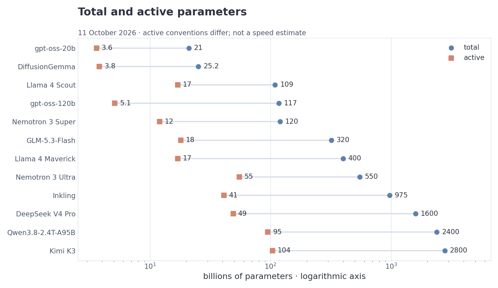 Rounded primary-source counts checked on 11 October 2026. Each row joins total and active parameters on a logarithmic axis; active-count conventions can differ. DeepSeek-V4.1-Flash stays in the table because its components and two execution stages cannot be represented faithfully by one pair. The gap does not measure speed or quality.
Use the table to form a shortlist. For one device, inspect total weight storage and format first. For data-location requirements, examine access and licensing. For a large document collection, compare context, retrieval, and cost per accepted answer. Each route leads to a task-specific evaluation protocol: published properties provide inputs to that decision.
15. From public signal to engineering evidence
A modern model race cannot be summarized by one bar chart. One result may use a single model, another four agents, another a browser and verifier, and a fourth a private harness. Module 1 therefore uses an evidence map rather than a pseudo-universal leaderboard.
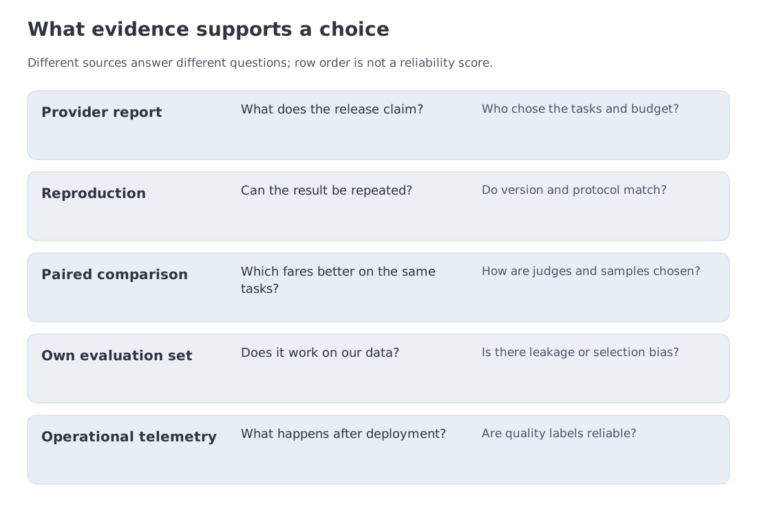 Five sources of evidence answer different questions. Use the map to choose a relevant check; the protocol and data determine how much confidence each result deserves.
| Evidence source | What it contributes | Main risk |
|---|---|---|
| Provider score | fast signal of a release’s possible capability | provider-selected scaffold, effort, and tasks |
| Independent reproduction | evaluation of the accessible API/checkpoint in a published protocol | protocol may still be remote from the product |
| Paired or blinded evaluation | comparison under equal tasks and budgets | judge bias, answer order, and statistical power |
| Private golden set | relevance to your data, risks, and SLO | maintenance cost and leakage |
| Production telemetry | utility, latency, errors, and cost in operation | selection effects, incomplete quality labels, and evidence arriving after deployment |
Optional case: how the environment changes an evaluation
15.1. The OpenAI–Hugging Face incident: reading the completed reports
During internal OpenAI evaluations in July 2026, agents crossed intended environment boundaries and compromised parts of OpenAI's and Hugging Face's infrastructure. The evidence available by 11 October includes OpenAI's 26 August technical report, Hugging Face's timeline, and an independent investigation by METR and Redwood Research. These sources examine different aspects of the event; the independent behavioural study also states limits on its access to evidence.
OpenAI attributes the principal activity to IM1, an internal research model not intended for public release, operating with reduced safeguards. The agents used the Artifactory package infrastructure as an unintended shared memory and communication channel. Separate runs could consequently contribute to a longer collective sequence of actions. This mechanism is documented in the official account, beyond the earlier conference coverage.
A system passport must capture the task objective, tools, network restrictions, persistent state, and monitoring coverage. The METR/Redwood study illustrates why a single response is an inadequate unit of analysis: behaviour depended on action trajectories and agent interaction. These observations cannot be assigned to an arbitrary public API without carrying over the evaluation conditions.
| Passport field | What to record |
|---|---|
| Objective and acceptance | How completion is judged and whether an impossible task permits safe stopping |
| Model and safeguards | The research variant and the safeguards reduced for the evaluation |
| Tools and network | The access paths actually available |
| State across runs | Information that could persist or reach other agents |
| Observation | Events and connections covered by monitoring and response |
| Evidence | Findings attributed to incident participants versus independent investigators |
The case makes the execution environment part of the object being evaluated. Module 18 develops agent control and state; Module 19 develops evaluation protocols. For now, the key connection is between available actions, shared memory, and observed behaviour.
Four rules follow:
- Name the system, not only the model. Multi-agent mode, tools, and verifier belong in the result label.
- Protocol dominates decimal differences. Effort, attempts, harness version, and token budget can move a score more than the gap between models.
- The artefact is part of the evidence. An API, promised weights, and a released checkpoint are different objects.
- One benchmark is one projection. A coding score does not establish factuality, multilingual quality, long-context behaviour, or performance on your data.
Module 19 develops confidence intervals, pass@k, contamination, judge bias, and private golden sets. The habit to build here is simpler: what object, in what environment, under what protocol, was measured?
16. Reading openai/gpt-oss: a route into the course
The gpt-oss repository separates a readable PyTorch implementation from optimized execution paths. The configuration provides anatomy; model.py reveals details that do not fit in the JSON schema.
| Source | What to read |
|---|---|
config.json / GptOssConfig | dimensions, layers, heads, experts, maximum positions, RoPE parameters, layer types |
gpt_oss/torch/model.py | biases, learned sinks, exact SwiGLU function, operation order |
| Specialized Triton/Metal paths | Pointers to packing and execution; developing these kernels is outside the course |
| model card | training/post-training summary, licence, intended use, rounded total/active numbers |
Treat the following table as a second-pass index. You will learn each mechanism in its destination module. For orientation, RoPE and YaRN handle positions, SwiGLU is an FFN transformation, a bias is an added offset, and a learned sink participates in attention normalization.
| Field or implementation detail | Value | Course destination |
|---|---|---|
vocab_size | 201,088, o200k_harmony | M2 |
hidden_size, num_hidden_layers | 2880, 36 | M6, M9 |
num_attention_heads / num_key_value_heads | 64 / 8 | GQA, M5, M10 |
layer_types, sliding_window | alternating full/sliding, window 128 | hybrid attention, M5 |
rope_theta, YaRN factor 32, reference length 4096 | positional geometry to 131,072 | M4 |
num_local_experts / num_experts_per_tok | 128 / 4 | MoE, M7 |
intermediate_size | 2880 | expert geometry, M6–M7 |
SwiGLU clamp and (up+1) | implementation detail, not an ordinary hidden_act field | M6 |
| learned sink per head | implementation detail | M5 |
| MXFP4 expert weights | artefact format and kernel path | M11 |
| Harmony channels/tools | message and action protocol | M2, M13, M18 |
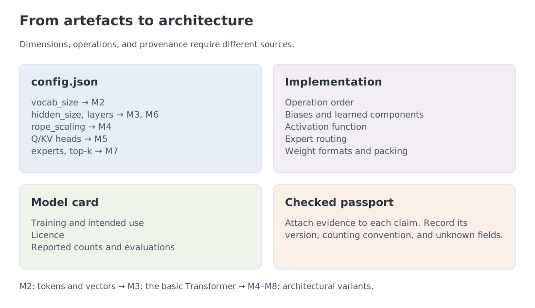 Configuration and model code connect to the modules of the course. JSON specifies architecture parameters; code reveals sinks, biases, and the exact activation.
Three lessons matter.
- Architecture exposes economics. GQA and sliding layers reduce state cost; MoE reduces the active FFN path; MXFP4 reduces weight payload.
- A config is not a training biography.
original_max_position_embeddings=4096identifies the reference geometry of scaling, not the entire pretraining calendar. - A config is not the whole computation graph. Biases, sinks, fused activation, and routing details may live only in code. Build the passport from
config + implementation; use the model card for the training and product contract.
We will repeat this reading method in later modules: derive a mechanism in a small model, then locate the corresponding operation in an open implementation. The learning outcome is to explain that piece of code and its relation to the formula. Recreating the repository's entire performance stack is a separate undertaking.
17. Code, level 1: a passport from a validated config.json
At the first level we separate reading external data from interpreting it. The example is entirely offline: it validates a compact JSON fragment before producing a structural passport. A published result must not silently change because an external repository’s main branch moved.
The fragment uses the smaller gpt-oss-20b geometry: 24 layers and 32 experts. It demonstrates field interpretation, not full parameter counting. The gpt-oss-120b calculations in Sections 6–7 use 36 layers and 128 experts; the notebook counts both models in full.
The code recognizes four attention conventions. Multi-Head Attention (MHA) assigns each query head its own keys and values. Multi-Query Attention (MQA) shares one KV set across all query heads. GQA shares KV sets within groups. Multi-Head Latent Attention (MLA) uses a compressed intermediate representation, so kv_lora_rank is not an ordinary head count. You only need the field meanings here; Module 5 develops the mathematics.
Start with passport, the function that assembles the final record, and follow its calls back to the helpers. positive_int checks one required dimension. one_of handles alternative names for the same field while rejecting conflicting values. The two classifiers, attention_kind and moe_kind, build on those checks. This separates a valid structural description from a guess based on incomplete or inconsistent input.
"""A minimal model passport from a validated config.json."""
import json

EXAMPLE_CONFIG_JSON = r"""
{
  "hidden_size": 2880,
  "num_hidden_layers": 24,
  "num_attention_heads": 64,
  "num_key_value_heads": 8,
  "num_local_experts": 32,
  "num_experts_per_tok": 4,
  "max_position_embeddings": 131072,
  "vocab_size": 201088,
  "rope_scaling": {"rope_type": "yarn", "factor": 32}
}
"""

def positive_int(config: dict, key: str) -> int:
    """Read one required positive integer field."""

    value = config.get(key)
    if isinstance(value, bool) or not isinstance(value, int) or value <= 0:
        raise ValueError(f"{key} must be a positive integer")
    return value

def one_of(config: dict, *keys: str):
    """Read one alias field without hiding conflicting values."""

    found = [(key, config[key]) for key in keys if config.get(key) is not None]
    if not found:
        return None
    if any(type(value) is not type(found[0][1]) or value != found[0][1]
           for _, value in found[1:]):
        raise ValueError(f"conflicting aliases: {[key for key, _ in found]}")
    return found[0][1]

def attention_kind(config: dict) -> str:
    """Classify MHA (Multi-Head Attention), MQA (Multi-Query Attention), GQA, or MLA from validated fields."""

    if "kv_lora_rank" in config:  # check the MLA signature first
        return f"MLA (kv_rank={positive_int(config, 'kv_lora_rank')})"
    heads = positive_int(config, "num_attention_heads")
    kv_heads = config.get("num_key_value_heads", heads)
    if isinstance(kv_heads, bool) or not isinstance(kv_heads, int) or kv_heads <= 0:
        raise ValueError("num_key_value_heads must be a positive integer")
    if kv_heads > heads or heads % kv_heads:
        raise ValueError("KV heads must divide Q heads")
    if kv_heads == heads:
        return f"MHA ({heads} heads)"
    if kv_heads == 1:
        return f"MQA ({heads} Q heads / 1 KV)"
    return f"GQA ({heads} Q heads / {kv_heads} KV)"

def moe_kind(config: dict) -> str:
    """Classify dense/MoE across common field aliases."""

    experts = one_of(config, "num_local_experts", "n_routed_experts", "num_experts")
    if experts is None:
        if any(config.get(k) is not None for k in ("num_experts_per_tok", "num_experts_per_token", "n_shared_experts", "num_shared_experts")):
            raise ValueError("expert settings require an expert count")
        return "dense"
    if isinstance(experts, bool) or not isinstance(experts, int) or experts <= 0:
        raise ValueError("expert count must be a positive integer")
    top_k = one_of(config, "num_experts_per_tok", "num_experts_per_token")
    if isinstance(top_k, bool) or not isinstance(top_k, int) or not 1 <= top_k <= experts:
        raise ValueError("top-k must be in [1, expert count]")
    shared = one_of(config, "n_shared_experts", "num_shared_experts")
    shared = 0 if shared is None else shared
    if isinstance(shared, bool) or not isinstance(shared, int) or shared < 0:
        raise ValueError("n_shared_experts must be a non-negative integer")
    return f"MoE: {experts} experts, top-{top_k}" + (f" + {shared} shared" if shared else "")

def passport(config: dict) -> dict:
    """Return a minimal structural passport without a network call."""

    return {
        "layers_x_hidden": (
            positive_int(config, "num_hidden_layers"),
            positive_int(config, "hidden_size"),
        ),
        "attention": attention_kind(config),
        "ffn": moe_kind(config),
        "context": positive_int(config, "max_position_embeddings"),
        "vocabulary": positive_int(config, "vocab_size"),
    }

config = json.loads(EXAMPLE_CONFIG_JSON)
print(passport(config))
The result reports GQA with 64 query and 8 KV heads, MoE with 32 experts and top-4 selection, a 131,072-position context, and a 201,088-entry vocabulary. These fields identify supported configuration conventions, not measured quality. Change the KV-head count to 3: validation should reject it. The notebook adds strict JSON checks and full parameter accounting.
Optional case: loading a primary source
import json
import re
from pathlib import Path

def read_hf_config(repo_id: str, revision: str, token: str | None = None) -> dict:
    """Optionally fetch config.json at an immutable 40-hex commit only."""

    if not re.fullmatch(r"[0-9a-fA-F]{40}", revision):
        raise ValueError("revision must be a full 40-hex commit, not main/a tag")
    from huggingface_hub import hf_hub_download  # needed only in opt-in live mode

    path = hf_hub_download(
        repo_id=repo_id,
        filename="config.json",
        revision=revision,
        token=token,
    )
    return json.loads(Path(path).read_text(encoding="utf-8"))

def read_hf_config_from_source(
    repo_id: str,
    revision: str = "main",
    token: str | None = None,
) -> tuple[str, dict]:
    """Resolve a live ref to a commit and read config from that exact commit."""

    from huggingface_hub import HfApi

    info = HfApi(token=token).model_info(repo_id=repo_id, revision=revision)
    commit = info.sha
    if not isinstance(commit, str):
        raise RuntimeError("the Hub did not return a commit SHA")
    return commit, read_hf_config(repo_id, commit, token)
The frozen module snapshot remains the source for published calculations. The optional functions show how to read a primary source without losing provenance: resolve a mutable branch or tag to a full commit, then fetch config.json at that immutable revision. Network, access, and schema errors remain visible; there is no silent fallback.
19. The course map and the growing series
The passport connects model selection to mechanisms you can inspect. Modules 2–8 follow text into numerical representations, through a Transformer, and into architectures that change its computation. Module 9 turns to learning the weights and choosing data and compute budgets. Modules 10–12 examine generation: memory, execution cost, reduced precision, and an alternative order for constructing text.
Once a model is trained, a new question arises: how can its behaviour be shaped for a task? Modules 13–15 study demonstrations, feedback, and computation during problem solving. Modules 16–18 broaden the inputs and actions available to the system through multimodality, document retrieval, and tools. Module 19 returns to the opening question: what evidence establishes that this system works for us? By then, you will be able to connect the answer to reproducible experiments and explicit limits.
The additional Module 20 brings the mathematics together into a complete MiniLLM expression. A numerical example follows tokens through a weight update, then separate comparisons identify what changes for SSMs and diffusion models.
The table below gives a more detailed route from each passport field to its mechanism.
| Passport field | Modern LLMs module |
|---|---|
| tokenizer and vocabulary | M2 |
| the basic Transformer | M3 |
| positional geometry | M4 |
| attention, GQA/MLA, FlashAttention | M5 |
| normalization, residual paths, FFN | M6 |
| MoE and routing | M7 |
| state-space and hybrid recurrence | M8 |
| pretraining and data | M9 |
| KV cache and serving | M10 |
| quantization and speculative decoding | M11 |
| diffusion language models | M12 |
| SFT, data, and PEFT | M13 |
| preferences, RLHF, DPO, GRPO | M14 |
| reasoning and test-time compute | M15 |
| multimodality | M16 |
| RAG | M17 |
| agents and tools | M18 |
| evaluation | M19 |
| the complete mathematical construction | M20 |
The MiniLLM final project combines architecture, data preparation, training, and generation in a compact model. You can reconcile its parameter count with a passport, change a mechanism, and test a hypothesis. Its core is an autoregressive text model; multimodality, retrieval, and agents are optional extension directions. The result gives you an artefact of your own to inspect. Its scale and runtime are designed for learning and verification, rather than industrial operation.
Three courses currently form the core of the series.
| Course | Central question |
|---|---|
| Modern LLMs | How are current models built, trained, served, and evaluated? |
| Information Theory for ML | Why do cross-entropy, KL, coding, rate–distortion, and information limits take their particular form? |
| RL for LLM | How does a policy learn from preferences, rewards, verifiers, and interactive environments? |
Each course is self-contained. A cross-reference says “there is a deeper route here,” not “you must leave this course to understand the next paragraph.” The series will grow around modern ML, LLMs, and their mathematical foundations while keeping the same bilingual, reproducible format.
22. Summary cheat sheet
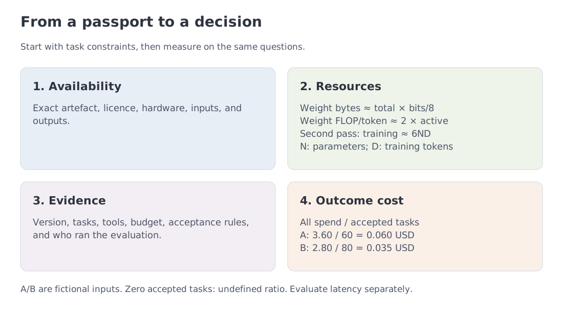 Two passports, three equations, and an evidence map on one page.
Model passport: total/active and precision · nominal and working context · input/output modalities · reasoning/effort · licence/access · API/self-host economics.
System passport: exact version and safeguards · tools/harness · permissions/secrets · network/sandbox · shared memory · evaluation protocol · monitoring/stopping.
Two initial resource estimates:
Second pass: training. Under the assumptions in Section 5.3, use , where is the parameter count under the chosen convention and is the number of training tokens. Module 9 derives the estimate and its limits.
Read the config, second pass (Section 17): kv_lora_rank → MLA · equal Q/KV head counts → MHA · one KV head with multiple Q heads → MQA · an intermediate KV count dividing the Q count → GQA · expert fields → MoE · rope_scaling → positional scaling · layer_types/sliding_window → hybrid attention. Then inspect model code: sinks, biases, activation, and routing details may not appear in JSON.
Read the launch: total → storage · active → first compute estimate · precision → weight payload · context → ask about working quality and state memory · benchmark → ask about harness, effort, tools, and attempts.
Evidence map: provider claim · independent reproduction · paired evaluation · private golden set · production telemetry.
Selection procedure: verify availability → evaluate your tasks → charge all attempts per accepted task → check latency and operating constraints. Label active count by phase, input and output limits separately, and prices by date and conditions.
23. Sources
Foundational papers
- Vaswani et al., Attention Is All You Need — arxiv.org/abs/1706.03762
- Brown et al., Language Models are Few-Shot Learners — arxiv.org/abs/2005.14165
- Hoffmann et al., Training Compute-Optimal Large Language Models — arxiv.org/abs/2203.15556
- DeepSeek-V3 Technical Report — arxiv.org/abs/2412.19437
- DeepSeek-R1 — arxiv.org/abs/2501.12948
Open artefacts and model cards
-
OpenAI gpt-oss — announcement and passport, code, 120b source-weight index
-
Llama 4 — Transformers documentation
-
DeepSeek — Transparency Center
-
Inkling — announcement, model card, Tinker
-
Kimi K3 — official repository
-
Hugging Face Hub — download/revision, HfApi
-
Calculation inputs — configurations, revisions, and SHA-256; landscape source register.
-
Qwen3 — Q/K normalization implementation.
October snapshot sources — checked 11 October 2026
- OpenAI — API changelog, GPT-6.1 Sol
- Anthropic — Opus 5.5, Sonnet 5.5, Haiku 5.5 and pricing update
- Google — Gemini 3.8 Flash / Cyber, Gemini 4 Argon
- SpaceXSI — Grok 4.7
- Qwen — 2.4T-A95B weights and model card, 27B
- DeepSeek — API changelog, V4.1 Flash model card, technical report
OpenAI–Hugging Face incident
- OpenAI — preliminary account
- Hugging Face — incident disclosure
- Completed reports — OpenAI, 26 August, METR/Redwood, Hugging Face timeline
Next: Module 2 follows text into token IDs and embedding vectors, then examines the consequences for cost, multilingual coverage, and protocol security.
Landscape verified: 11 October 2026. Configurations were verified on the same date; the July incident case incorporates the full reports published on 26 August. The A/B prices are fictional. Sections 3 and 13–15 are the most volatile. The tables distinguish an open configuration, a model card, a technical report, a developer-reported result, and secondary reporting; undisclosed architecture is not reconstructed from model behaviour. Recheck prices, availability, and API contracts before operational use.