Module 16. Multimodal LLMs: Vision, Audio, and Video
“Modern LLMs” course · Module 16 lecture · edition 2026.10.25
What this module is about. Imagine a user who attaches a screenshot, explains it with a voice note, and asks the system to locate the same event in a video. The user sees one task. The model sees three physical signals with different geometry, time scales, and output requirements. Each signal creates four design obligations: build a representation, compress it into an affordable budget, preserve the structure that matters, and decide which component will produce the answer.
We will first follow an image into a text answer, then add video and streaming speech. The necessary components emerge along that path: extracting features, connecting them to a language model, and reconstructing an output signal. This gives us a basis for comparing architectures by the work each component performs.
The worked examples connect geometry to systems cost: 576, 2,880, and 1,296 visual positions; 72, 360, and 162 MiB of image KV under one declared GQA geometry; symmetric InfoNCE on a four-pair batch; a dense-equivalent LLaVA-style training scenario; and a two-hour video that becomes millions of tokens under naive frame sampling. Each calculation is used to answer a systems question: where does the architecture pay for a modality, and what bottleneck appears next?
Prerequisites. Module 4 introduces multidimensional position schemes, Module 5 provides GQA and KV-cache geometry, Module 9 uses the training approximation, Module 10 separates prefill from decode, and Module 15 studies the cost of extra inference context. The necessary ideas are restated here, so the chapter is self-contained.
Reading routes
First reading. Follow the system in Sections 1–4, count the cost of one image in Sections 6–7, then connect resolution, video, and speech in Sections 9–12. Finish with Sections 15–17 and 20. Model names in the historical overview are signposts; their mechanisms are introduced later. At this stage, a contrastive encoder means an encoder trained to give matching images and captions nearby vectors.
Second reading. Work through the loss in Section 5, connector training in Section 8, and the executable experiments in Sections 13–14. Use Section 19 to check whether you can explain each result from its assumptions, including the complete pixels-to-answer experiment.
Reference use. Sections 6–8 and 11 hold the numerical examples, Section 16 records dated source evidence, and Section 17 provides a configuration-reading procedure. The teaching video budget uses exactly 256,000 positions; a vendor's “256K” label may refer to a different exact limit.
1. Motivation: every modality creates a new budget
A text prompt already arrives in the model’s native currency: tokens. Pixels, waveforms, and video frames do not. They must first be converted into sequences or memories that a language-centered system can consume.
That conversion is not a neutral preprocessing step. It decides what evidence survives, how many positions are created, whether spatial and temporal relationships remain visible, and which decoder can later produce an answer.
A model connecting vision and language is a vision-language model (VLM). Multimodal systems may also support audio and video.
The word multimodal therefore covers at least three capabilities:
- Perception: accepting images, video, or audio as context.
- Cross-modal reasoning: combining evidence across those inputs.
- Generation: emitting speech, images, or another media stream rather than text alone.
A model may be strong at one and weak at another. A vision-to-text assistant can read charts without having an image generator. A unified image model may synthesize convincing pictures yet struggle with tiny text. A live speech system may expose one conversational endpoint while relying on separate internal components for understanding and audio production.
Throughout the chapter, we will track four design obligations.
- Representation: what object replaces the raw physical signal?
- Budget: how many positions, bytes, and operations does that object require?
- Structure: how are space and time encoded after compression?
- Output: which component generates text, pixels, or streaming audio?
The obligations interact immediately. If one image becomes 576 decoder positions, it lengthens prefill and may contribute 576 entries to every self-attention KV cache. At one frame per second, a two-hour video represented at 576 positions per frame exceeds four million positions before the user’s text is added.
This gives the chapter its central question:
How does an architecture turn physical evidence into a computational object, and which new constraint does that choice create?
A capability label such as “vision supported” cannot answer it. We need the processor, encoder, fusion topology, state layout, and output path.
2. Four families, four places to draw the boundary
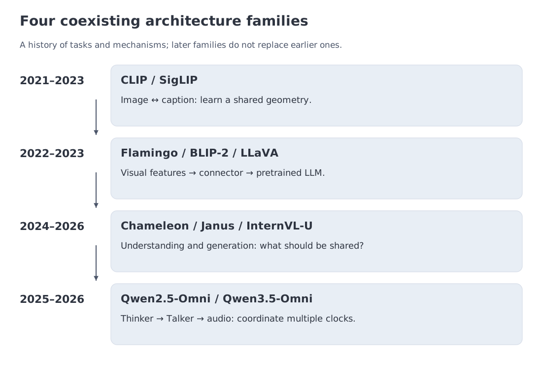 Four architectural lines: CLIP/SigLIP alignment, connector-based VLMs, unified understanding and generation, and omni systems with streaming audio. The lines overlap rather than replace one another.
The field does not form a clean staircase from “old modular system” to “new native model.” Each family moved a different boundary.
The earliest boundary was semantic. CLIP aligned image and text encoders so that paired items occupied nearby regions of one embedding space. SigLIP changed the objective while preserving the two-tower design. These encoders made retrieval and zero-shot transfer practical, but they did not answer users in natural language.
Connector-based systems moved the next boundary: instead of rebuilding language competence, Flamingo, BLIP-2, and LLaVA attached visual features to an existing LLM. The design was attractive because the language backbone could remain largely intact. Its new question was quantitative: how many visual positions reach the decoder, and where are they stored?
Unified understanding-and-generation systems moved the boundary again. Chameleon placed discrete text and image tokens in one autoregressive stream. Janus kept one Transformer but separated visual representations for understanding and generation. InternVL-U let a multimodal language model provide reasoning and conditioning while an MMDiT head handled image generation and editing. These systems share an external interface, but they disagree about what should be common internally.
Omni systems introduce a temporal boundary. Qwen2.5-Omni and Qwen3.5-Omni coordinate text, images, audio, and video while producing text and streaming speech. Thinker–Talker is explicitly multi-component: one part integrates evidence and language, another converts hidden state into an audio-token stream.
The coexistence is the point. A contrastive encoder is still the right object for retrieval. A connector can reuse a strong language model at a much smaller training budget than training all components from scratch; it is not universally the cheapest deployment. A unified generator is useful when text and pixels must share context. An omni system is designed around streaming clocks. Rather than asking which family is “most advanced,” ask which representation, memory, and output boundaries the design chooses to share.
3. Three older ideas provide the mental model
VLMs become easier to reason about when we connect them to three older engineering traditions.
Metric learning organizes semantics
Siamese and dual-encoder systems learn a geometry in which related objects are close and unrelated objects are far apart. CLIP applies that idea to image–caption pairs. The resulting visual vectors are not “words,” but they are already organized by concepts that language can name.
This explains why a small connector can sometimes be effective. It does not start from raw pixels; it starts from representations that already distinguish meaningful visual content. This does not require individual coordinate axes to correspond to named concepts.
Vision Transformers turn area into sequence length
ViT divides an image into patches, projects each patch, and sends the resulting sequence through a Transformer. For image height , width , and square patch size ,
when both dimensions divide exactly. The equation exposes a basic systems fact: doubling both spatial dimensions roughly quadruples the number of patch positions. Visual token count is tied to area, not only to semantic complexity.
Signal-processing pipelines separate rates and responsibilities
Speech systems long separated acoustic encoding, language modeling, and waveform decoding. A contemporary multimodal model often makes the same separation trainable end to end: modality-specific encoders compress raw signals, a language-centered module reasons over them, and specialized decoders reconstruct speech or images.
End-to-end training therefore does not imply one homogeneous network or one token rate. Jointly trained modules may still use different losses, temporal resolutions, and state layouts. That observation will recur throughout the chapter: specialization is often how a system avoids forcing semantic understanding, pixel fidelity, and streaming latency into one representation.
4. The first design: encoder, connector, language decoder
Start with a single image question. The system must extract visual evidence, translate that evidence into a form the language model can use, and generate a response. The most legible VLM architecture assigns those jobs to three components.
- A vision encoder converts pixels into a sequence of features.
- A connector adapts feature width, count, or access pattern to the LLM. A multilayer perceptron (MLP) stacks linear maps and nonlinearities; learned-query modules such as Q-Former and Perceiver Resampler can also shorten the feature sequence.
- A language decoder combines visual evidence with the prompt and generates text.
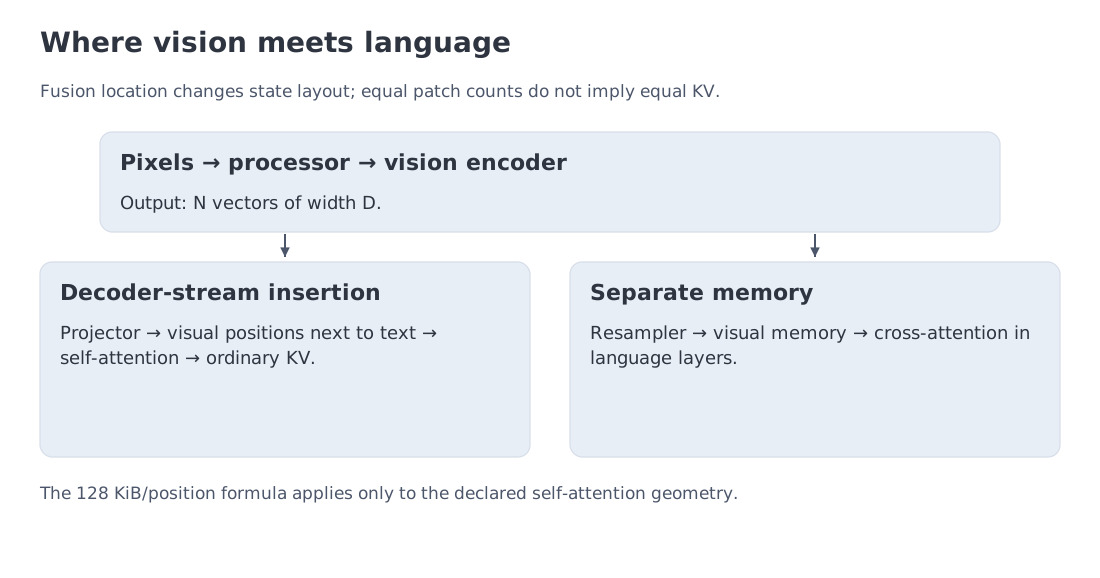 A modular VLM: image processing and encoding produce visual features; a connector changes width or count; the language decoder consumes the result either in its token stream or through cross-attention.
The connector’s location determines where the visual cost appears.
Modules 2–3 used “token” for a discrete ID that selects a row from an embedding table. A visual token often means a continuous feature vector occupying one sequence position. The projector can supply that vector directly, without assigning it an ID in the text vocabulary. Both occupy positions, but their representations are obtained differently. Section 10 will introduce visual codecs that do produce discrete indices.
Decoder-stream insertion. Projected visual vectors become ordinary positions next to text embeddings. The design is simple and uses the decoder’s existing self-attention machinery, but every visual position lengthens the sequence and may create K/V state in every layer. Section 7 uses this contract.
External visual memory. Flamingo-style cross-attention keeps visual features outside the text stream. The language stack periodically reads them. Sequence length pressure is reduced, but the model now carries a second attention path and a separate visual memory.
Compression before the LLM. A Q-Former or resampler maps many patch features into a smaller set of learned queries. The connector spends compute to reduce the number of expensive decoder positions.
The modular design also changes deployment choices. The vision encoder can be replaced, placed on another device, or cached when several questions refer to one document. But before exploiting those options, we need to understand what the encoder learned and how many positions its processor creates. Sections 5–7 make both quantities explicit.
5. CLIP, SigLIP, and worked example C: reading InfoNCE numerically
A small connector can work because the vision encoder has already been shaped by language supervision. InfoNCE makes that statement precise.
Let normalized image embeddings form matrix , normalized text embeddings form , and define
For image-to-text retrieval, one row of the similarity matrix is divided by temperature and normalized with softmax. Symmetric CLIP loss averages the image-to-text and text-to-image cross-entropies.
Write the batch as : paired examples, embedding width , and unit Euclidean norm for each row. Matching indices identify the supervised pair. With temperature , the complete objective is
Read the first denominator across captions and the second across images. The two retrieval problems share the same batch but need not have the same loss: in general the similarity matrix is not symmetric. Temperature scales the competition without changing the embedding vectors.
Consider four matched pairs with diagonal similarity 0.8 and off-diagonal similarity 0.2. At , the positive logit is 8 and each negative logit is 2. The matched probability is
so the loss is
At , the probability falls to 0.525325 and the loss rises to 0.643738. Temperature has not changed the underlying similarities; it has changed how sharply they compete.
If every similarity is equal, softmax is uniform and the loss is . For , the random-matching reference is 1.386294. It is a reference, not a mathematical floor: an actively misordered matrix can be worse.
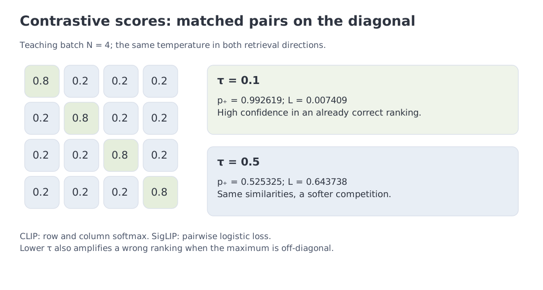 The 4×4 similarity matrix at two temperatures, together with the CLIP/SigLIP distinction. The numbers belong to the teaching batch, not to a published training curve.
In a large CLIP batch, each item competes with negatives in the corresponding direction. More negatives help only up to a point, and the global softmax denominator complicates distributed training.
SigLIP replaces row-wise global normalization with independent sigmoid losses on pairs. One loss term no longer requires a global softmax denominator, which simplifies implementation and permits different positive/negative sampling strategies. The examples included in a batch still affect the learned geometry.
SigLIP assigns each pair a label and a logit , using a positive scale and a bias . Its pair loss is , evaluated as softplus(-y*z). The original batch objective sums the pair terms and divides by ; averaging over all pairs changes the scale. Pairwise logistic loss removes the shared softmax denominator, not every dependence on batch-size scaling or negative sampling.
The temperature experiment also has a condition worth testing: the matched pair must already rank first. If a wrong caption has the highest score, lowering the temperature makes the error more confident and raises the loss. Semantically equivalent captions can become false negatives, so supervision quality remains part of the mechanism.
Contrastive learning explains semantic compatibility. It does not determine how many visual features reach the decoder. That is the next accounting step.
6. Worked example A: three ways to spend visual tokens
The first bill for an image is issued by the processor, before any language-layer computation. Patch size, tiling, and merging decide how many positions the rest of the system must carry.
For a 336×336 image with 14×14 patches,
positions are produced. This counts the spatial patches of CLIP ViT-L/14@336 used by LLaVA-1.5. The encoder's extra CLS position, which aggregates image information, is not one of these 576 patches.
The module’s 2,880-token case is deliberately different from one 672×672 grid. It represents four local 336×336 tiles plus one global thumbnail:
Tiling preserves local detail by paying for several views of the image.
For a Qwen2-VL-like 1008×1008 input, 14-pixel patches create
spatial features. A 2×2 spatial merger combines four neighbors into one decoder-facing token:
This strategy retains high-resolution processing early and compresses the sequence before the expensive language layers.
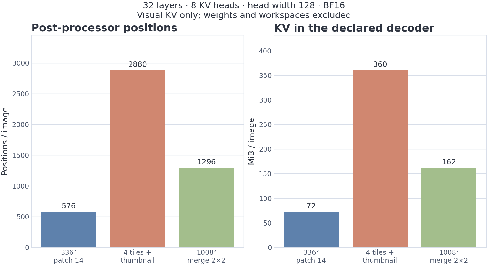 Three explicitly different visual-processing contracts and their KV cost under one teaching GQA geometry.
The examples show why raw input resolution is not a sufficient passport field. A processor may preserve aspect ratio, round to a valid grid, enforce pixel limits, add overlapping tiles, include a thumbnail, use temporal patches, or insert separator tokens.
Patch arithmetic is therefore a first sanity check. The authoritative count comes from the actual processor and model configuration. Once that count is known, we can ask where the positions live and how much state they create.
7. Worked example B: when images create ordinary decoder KV
Consider a language decoder with 32 layers, 8 KV heads, head dimension 128, and bf16 keys and values. One cached position costs
If projected visual features enter ordinary decoder self-attention, image positions use the same accounting as text.
| Representation | Visual positions | KV per image |
|---|---|---|
| LLaVA-336 | 576 | 72 MiB |
| four local tiles + thumbnail | 2,880 | 360 MiB |
| 1008 px with 2×2 merger | 1,296 | 162 MiB |
The table connects processor design to serving cost. The tiled input carries five times the KV of the 336 case. The merged case exposes the encoder to a higher-resolution input and uses less than half the tiled scenario's decoder KV. Whether useful detail survives learned compression is an empirical question.
Suppose 15 GiB of an 80-GiB device is occupied by weights and, unrealistically, every remaining byte is available for image KV. The resulting upper bounds are 924, 184, and 410 images.
They are intentionally optimistic. Real serving also needs text context, output tokens, activations, allocator reserve, temporary workspaces, and memory for the vision encoder.
More importantly, the formula is architectural. It applies when visual positions pass through decoder self-attention and their K/V is retained in the stated format. Resampling can reduce the number of positions without changing their per-position KV formula; the resampler itself adds separate work. Pruning may likewise change which positions remain. A different state layout, such as cross-attention or recurrent memory, requires its own accounting.
The connector therefore determines more than compatibility. It decides where the cost of visual memory is paid.
8. Connectors control where computation happens
Sections 6 and 7 exposed the cost of preserving visual detail: more patches can become more decoder positions and more KV state. The connector decides whether that cost remains in the LLM sequence, is compressed first, or is moved into a separate memory path.
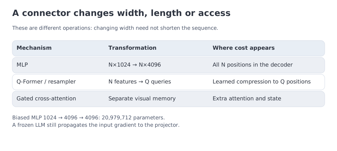 MLP projection, Q-Former/resampling, and gated cross-attention change different resources: width, position count, or the location of visual state.
MLP projection: adapt width, keep the positions
LLaVA-1.5 uses a two-layer MLP between CLIP features and the LLM width. For 1024→4096→4096 with biases,
parameters are trainable in the projector. The MLP changes feature space, not sequence length: 576 image patches normally remain 576 visual positions in the decoder.
Keeping position count does not guarantee preserving all information: the MLP is a learned transformation, not necessarily an invertible map. It transfers the full position count into the language stack.
Q-Former or resampler: purchase compression before the decoder
BLIP-2 uses learned queries that cross-attend to a larger visual feature set. The number of output queries becomes an explicit information bottleneck. A high-resolution image can still produce a short decoder sequence.
The saved decoder cost is paid in two ways: extra connector computation and the risk that a small query set omits a fine detail needed by the task. Query count is therefore both a systems parameter and an assumption about evidence complexity.
Gated cross-attention: keep visual state beside the text stream
Flamingo leaves visual features in a separate memory and inserts gated cross-attention into the language stack. This avoids treating every image feature as an ordinary text position, but introduces a second state path and modifies the decoder architecture.
Now consider the module’s LLaVA-style training scenario:
- 558K alignment pairs at an assumed 600 tokens each;
- 665K multimodal instruction examples at an assumed 1,000 tokens each.
In , is the language-model parameter count, is the number of processed positions, and is an approximate operation count. Model FLOP utilization (MFU) supplies the assumed useful fraction of peak throughput: TFLOP/s here. Encoder work and quadratic attention operations are not separately included.
For one common accounting convention, apply to a 7B model in both phases and divide by 990 TFLOP/s at MFU 0.4. The two estimates round to 9.864 and 19.592 hours. Adding before rounding gives a total of 29.455 H100-equivalent hours.
That number is a dense-equivalent teaching scenario, not measured LLaVA wall time. Frozen LLM weights need neither weight gradients nor optimizer state during alignment, but backward computation through input activations is still required to train the projector. Wrapping the whole LLM in no_grad() would sever that path. Counting only the projector's 21 million parameters therefore also understates the work. Conversely, real training includes data loading, communication, and imperfect utilization.
The calculation answers a narrower architectural question: why can attaching trained components be orders of magnitude cheaper than multimodal pretraining from scratch?
A connector still cannot recover detail discarded by image preprocessing. As soon as OCR, diagrams, or fine-grained documents matter, the design pressure moves upstream to resolution. The next section follows that pressure and shows how input dimensions and processing policy make request cost variable.
9. Dynamic resolution makes compute depend on image geometry
A fixed square resize works well when the relevant object is large. It is destructive when the evidence is tiny text in a screenshot or a dense technical diagram. A larger resolution can preserve more of that detail, but also spends more resources on inputs that do not benefit from it.
Qwen2-VL’s Naive Dynamic Resolution makes the processor respond to the actual image dimensions within a bounded range. Images approximately retain aspect ratio subject to grid rounding and become sequences of different lengths. The rule uses geometry and pixel limits, not a semantic judgment that one image is simpler than another. Spatial merging then reduces the number of positions before the language decoder.
Variable length solves one problem and exposes another: positions must retain their meaning when text, image regions, and video frames are interleaved. M-RoPE (Multimodal Rotary Position Embedding) assigns temporal, vertical, and horizontal coordinates rather than treating the sequence as one undifferentiated line. Text advances coherently across the axes; an image occupies a two-dimensional grid; video adds time.
Qwen2.5-VL strengthened explicit temporal grounding. Qwen3-VL combines improved interleaved M-RoPE, DeepStack injection of multi-level ViT features, and text-aligned timestamps within a native 256K interleaved context. The architectural sequence is causal: geometry-dependent processing changes sequence length; interleaving mixes evidence sources; positional encoding must preserve their addresses.
InternVL follows another route to detail. It tiles large images and often adds a global thumbnail. The thumbnail preserves scene-level context while local tiles recover fine structure. The InternVL3.5-Flash variant adds ViR: a learned router selects 256 or 64 decoder positions from each tile's 1,024 encoder positions. This is content-dependent compression. Decoupled deployment of the vision and language components is a separate systems technique in the family.
Both approaches make compute a property of the input, not merely the number of images. Capacity planning now needs distributions of post-processor area, tile count, visual sequence length, and packing efficiency.
This also prepares the next question. A semantic encoder can discard nuisance detail when the output is text. A model that must generate or edit images may need exactly that discarded detail. “Unified” modeling begins where those objectives collide.
10. Unified output reveals a conflict between semantics and fidelity
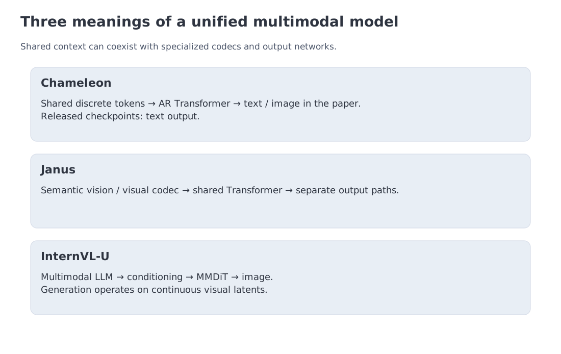 Chameleon, Janus, and InternVL-U share different things: discrete tokens, a Transformer backbone, or a language-centered reasoning context connected to an image-generation head.
Image understanding rewards invariance. To answer “what is in the scene?”, the representation should ignore many pixel-level changes. Image generation and editing reward the opposite property: texture, layout, and high-frequency details must remain recoverable.
The term unified therefore needs a qualifier. Are tokens unified? Is the Transformer shared? Is training joint? Or is only the product interface unified?
Chameleon: one discrete stream
Chameleon tokenizes images with a visual codec and trains one Transformer over mixed text and image token sequences. It is the most literal early-fusion design: the research model can continue in either modality. Meta's released Chameleon checkpoints expose text output; the paper's image-generation capability is not a capability of those released checkpoints.
The simplicity concentrates the conflict in the codec. Strong compression helps sequence length and semantic abstraction, while high-fidelity generation needs detailed visual codes. One representation must serve both.
Janus: share sequence modeling, split visual encoders
Janus uses separate visual paths for understanding and generation while keeping a shared Transformer. The understanding encoder can emphasize semantic invariance; the generative path can preserve the information required by an image decoder.
Unification has moved upward—from the image representation to the reasoning backbone and shared context.
InternVL-U: reason jointly, render with a specialized head
InternVL-U lets a multimodal LLM handle understanding and reasoning, then conditions a Multimodal Diffusion Transformer (MMDiT) head for image generation and editing. The system is unified at the level of task interpretation and context, not at the level of the pixel-generation mechanism.
The examples lead to a durable principle:
A unified user contract does not require one internal representation.
The more strongly modalities differ in semantic abstraction, precision, and output rate, the more useful specialized paths can become. Video adds another dimension to this conflict: before preserving detail, the system must decide which moments deserve representation at all.
11. Worked example E: video is an information-selection problem
An image has a spatial price. Video multiplies it by duration. Treating every frame as another image quickly turns context length into the dominant constraint.
A two-hour video sampled at one frame per second contains 7,200 frames. At 576 positions per frame, naive representation requires
visual tokens—more than sixteen times a 256K context before text is included.
Reserve 4,000 positions for the prompt and answer. The remaining visual budget is 252,000 tokens.
Without merging,
frames fit, or one frame every 16.48 seconds.
At 144 tokens per frame after a 2×2 merger,
frames fit, or one every 4.11 seconds.
Here K means 1,000. The quoted 16.48 and 4.11 seconds are inverse sampling densities, . The notebook includes both endpoints of the 7,200-frame sequence, so mean spacing between retained timestamps is : 16.5115 and 4.1161 seconds. Rounded indices produce unequal neighboring gaps. Density and timestamp spacing should not be reported as the same quantity.
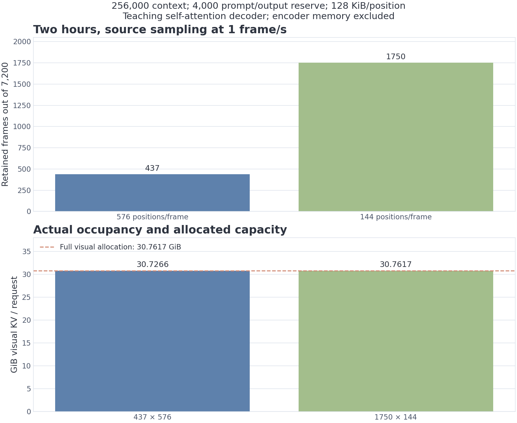 The scenario shows why video systems need temporal compression. It is not a reconstruction of any particular processor.
At 128 KiB per decoder position, the 252K visual budget alone creates 30.7617 GiB of KV; the full 256K context creates 31.25 GiB in the module’s 8B GQA geometry.
Whole frames do not necessarily fill the allocation. With 437 frames, actual visual occupancy is positions or 30.7266 GiB. Adding the full text reserve gives 255,712 positions and 31.2148 GiB, leaving 288 positions unused by frames. At 144 positions per frame, 1,750 frames fill the visual allocation exactly. Reserving future output capacity does not mean its KV has already been materialized.
The real question is not merely whether the context is large enough. It is which events deserve representation. Uniform sparse sampling can miss a short but critical event. Dense sampling preserves it while displacing other evidence. Practical systems therefore combine variable frame rate, temporal patching, near-duplicate removal, key-event selection, local temporal attention, hierarchical summaries, or external memory.
A context-window number does not tell us what survived the selection policy. The Qwen3.5-Omni report, for example, states more than ten hours of audio but 400 seconds of 720p video at one frame per second. Different modalities run at different effective token rates even within one system.
Video therefore introduces an evidence-selection obligation. Images ask how much detail to preserve; video first asks which moments should receive tokens at all. Streaming speech adds a second clock: the signal keeps arriving while output audio advances at its own rate.
12. Thinker–Talker: coordinating two clocks
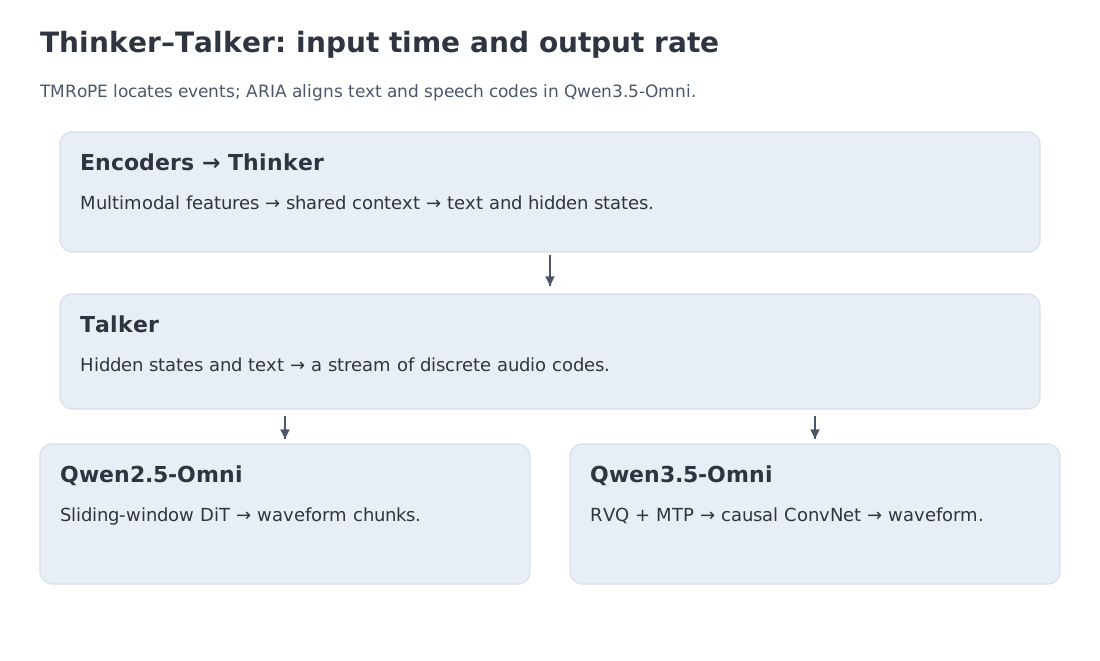 The Thinker integrates multimodal evidence and generates language-level state; the Talker emits streaming codec tokens. TMRoPE locates input events, while ARIA coordinates output rates.
Video introduced time on the input side. Live speech creates a second timing problem: text tokens, audio-codec tokens, and waveform packets are produced at different and variable rates. An omni system must know both when evidence occurred and how to coordinate its outputs.
Before following the two modules, distinguish the objects they exchange. A waveform is a sequence of amplitude samples. An acoustic frame is a short time window from which spectral features can be computed. Its feature vector is continuous, not a vocabulary ID. An encoder may combine several frames before passing a lower-rate sequence to the language module.
A neural audio codec provides a route back to sound. Its encoder produces vectors; a vector quantizer replaces them with indices into a codebook, a learned table of representative vectors. Those indices are discrete audio codes. The decoder uses the selected vectors to reconstruct an approximate waveform. Codebook entries need not correspond to words or phonemes, and one temporal frame may carry several codes. Section 15 counts feature positions and codec codes separately.
Qwen2.5-Omni offers a clear division of labor.
The Thinker consumes text, images, video, and audio and produces text tokens and hidden representations. Its visual and audio encoders can process blocks for streaming input. TMRoPE (Time-aligned Multimodal RoPE) addresses the input clock by assigning compatible temporal coordinates to audio and video while preserving visual spatial coordinates.
The Talker addresses output. It consumes Thinker representations and autoregressively produces discrete audio-codec tokens. A sliding-window Diffusion Transformer (DiT) reconstructs waveform chunks without waiting for the entire response, reducing time to first audio.
Qwen3.5-Omni retains the Thinker–Talker split, scales both components with Hybrid-Attention MoE, and adds ARIA (Adaptive Rate Interleave Alignment). ARIA is not another name for temporal position encoding. It coordinates text and speech streams whose tokenizers advance at different and changing rates. TMRoPE locates input events; ARIA synchronizes output production.
Follow the waveform path all the way through the version boundary. Qwen2.5-Omni uses sliding-window diffusion reconstruction. Qwen3.5-Omni instead uses residual vector quantization (RVQ): successive codebooks approximate what earlier books have left unexplained. A multi-token prediction (MTP) module predicts the residual codes, and a causal Code2Wav convolutional network reconstructs the waveform. It also supplements temporal position encoding with explicit timestamp strings. A shared Thinker–Talker name does not make those implementations identical.
The architecture is end to end without being monolithic. Joint training and one conversational interface can coexist with specialized modules and separate clocks.
That design determines what must be measured. Voice interaction needs more than one latency number:
- semantic answer quality;
- time to first audio packet;
- real-time factor : below one means generation is faster than playback;
- streaming stability and prosody;
- interruption latency and recovery;
- audio–video synchronization;
- voice similarity where cloning is supported.
Sections 13 and 14 now freeze the minimal mechanics—patch geometry, KV cost, and frame capacity—before we return to audio as a general temporal modality and compare public architectures.
13. Code level 1: geometry before frameworks
The functions below make three assumptions explicit: divisibility of image dimensions, decoder-KV geometry, and integer frame capacity.
"""Exact visual geometry and decoder-KV accounting; no implicit resize."""
from dataclasses import dataclass
from numbers import Integral

def positive_count(value):
    if isinstance(value, bool) or not isinstance(value, Integral) or value <= 0:
        raise ValueError("expected a positive integer")
    return int(value)

@dataclass(frozen=True)
class PatchLayout:
    grid_h: int
    grid_w: int
    merge: int
    visual_tokens: int

def patch_layout(height, width, *, patch=14, merge=1):
    height, width, patch, merge = map(positive_count, (height, width, patch, merge))
    if height % patch or width % patch:
        raise ValueError("image dimensions must be divisible by patch")
    gh, gw = height // patch, width // patch
    if gh % merge or gw % merge:
        raise ValueError("patch grid must be divisible by merge on both axes")
    return PatchLayout(gh, gw, merge, (gh // merge) * (gw // merge))

def kv_mib(tokens, *, layers=32, kv_heads=8, head_dim=128, bytes_per_value=2):
    tokens, layers, kv_heads, head_dim, bytes_per_value = map(
        positive_count, (tokens, layers, kv_heads, head_dim, bytes_per_value))
    return tokens * 2 * layers * kv_heads * head_dim * bytes_per_value / 2**20

def video_frames_fit(context=256_000, text_reserve=4_000, tokens_per_frame=576):
    context, tokens_per_frame = map(positive_count, (context, tokens_per_frame))
    if (isinstance(text_reserve, bool) or not isinstance(text_reserve, Integral)
            or not 0 <= text_reserve < context):
        raise ValueError("text_reserve must be an integer in [0, context)")
    return (context - int(text_reserve)) // tokens_per_frame
The lecture values follow directly:
assert patch_layout(336, 336).visual_tokens == 576
assert 5 * patch_layout(336, 336).visual_tokens == 2880
assert patch_layout(1008, 1008, merge=2).visual_tokens == 1296
assert kv_mib(2880) == 360.0
assert video_frames_fit() == 437
A real processor may explicitly resize or pad an image. Padded regions must be accounted for, but not every processor exposes a separate pixel mask; follow the actual interface contract. Silent integer truncation is not a preprocessing policy.
15. Audio is a continuous evidence stream
Audio makes the representation problem more demanding than a bounded image. A minute of speech creates a dense sequence of acoustic frames even when the transcript contains few words. The system must decide which properties of the waveform survive compression and which decoder will reconstruct the response.
Front end and encoder: define the evidence
A waveform becomes spectral features, learned representations, or discrete codec tokens. An automatic speech recognition (ASR) encoder such as Whisper prioritizes linguistic content. An omni system may also need prosody, environmental sounds, music, speaker attributes, and alignment with video.
The encoder therefore determines whether the language model receives only “what was said” or a richer description of how and when it was said.
Temporal compression: buy positions per second
Raw acoustic frames are too dense for direct LLM attention. Strided convolutions, pooling, or a neural codec reduce the rate. The trade-off mirrors spatial merging in vision: fewer positions lower cost but may discard phonetic detail, emotion, or timing precision.
Worked example F: seconds, frames, positions and codes
Start with six seconds of mono audio sampled at samples/s. The waveform contains amplitude samples, not 96,000 language tokens. Our teaching front end starts a 400-sample window every samples: a 25 ms window and a 10 ms hop. Window starts remain inside the signal; incomplete windows are padded on the right. This convention gives
Windows overlap, so multiplying their count by their width does not recover the original signal length. A real-input Fourier transform provides 201 frequency components per window. Keeping their magnitudes produces a feature matrix. This small spectral front end is inspectable; it is not a replica of Whisper's or Qwen's encoder.
Average successive groups of four frame vectors. The result has positions, each of width 201. For another input length, a final short group is averaged over its existing frames only. Position count and feature width are separate axes. If those positions are projected into the Section 7 decoder, their KV costs MiB, excluding front-end and projector work.
Now consider a separate codec scenario: 75 frames/s and eight codebooks with 1,024 entries each. Six seconds require 450 temporal frames and indices. Ten bits per index give a fixed-width payload of 36,000 bits, or bits/s. Headers, side information and entropy coding are outside this calculation; it is not a file-size prediction.
The 3,600 indices do not uniquely determine decoder KV. A system could flatten them into 3,600 sequential positions, combine each frame's eight codes into one representation, or use a separate predictor for some codebooks. EnCodec's implementation explicitly separates batch, codebook and time axes as [B,K,T]. That contract illustrates the distinction without prescribing the topology of an arbitrary omni model. EnCodec encoding and decoding
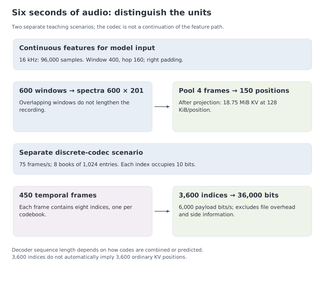 The teaching spectral front end and a separate multi-codebook scenario. Temporal frames, discrete codes and decoder positions are distinct counts.
Second reading: residual vector quantization. RVQ encodes what earlier codebooks have left unexplained. For input vector , the first book selects ; the second approximates , giving reconstruction . With , and , squared error falls from after the first book to after the second. These books are hand-written and each includes zero, so the nearest residual entry cannot do worse than making no correction. An arbitrary set of books does not guarantee this property. The same residual-encoding mechanism appears in the EnCodec implementation.
Representation size is also distinct from output speed. Suppose a speech decoder creates six seconds of audio in 2.4 seconds: . Its first packet might arrive after 0.18 seconds, a separate latency measure. These are illustrative timings, not measurements made by our spectral example. An average does not rule out playback gaps; streaming evaluation must inspect when individual chunks become ready.
Semantic reasoning: connect the stream to the task
A language-centered module interprets the evidence, answers a question, or plans an action. Temporal coordinates connect audio to video and text. When speech overlaps an event on screen, simple token order is not enough; simultaneous events need compatible time references.
Speech generation: return a stream, not a sentence
Language-level state is converted into codec tokens and then waveform. A live system must start speaking before the full answer is complete and must stop or recover when the user interrupts. The decoder therefore determines not only voice quality but also streaming delay and full-duplex behavior.
Qwen2.5-Omni and Qwen3.5-Omni document one such path; Step-Audio 2 provides another public audio-system report. Their latency figures are comparable only under matched language, hardware, buffering, and output contracts.
Audio brings the chapter back to its opening framework. A useful model passport must report the representation rate, compression, temporal geometry, memory path, and output decoder—not merely an “audio supported” badge.
16. Reading the public landscape by design axis
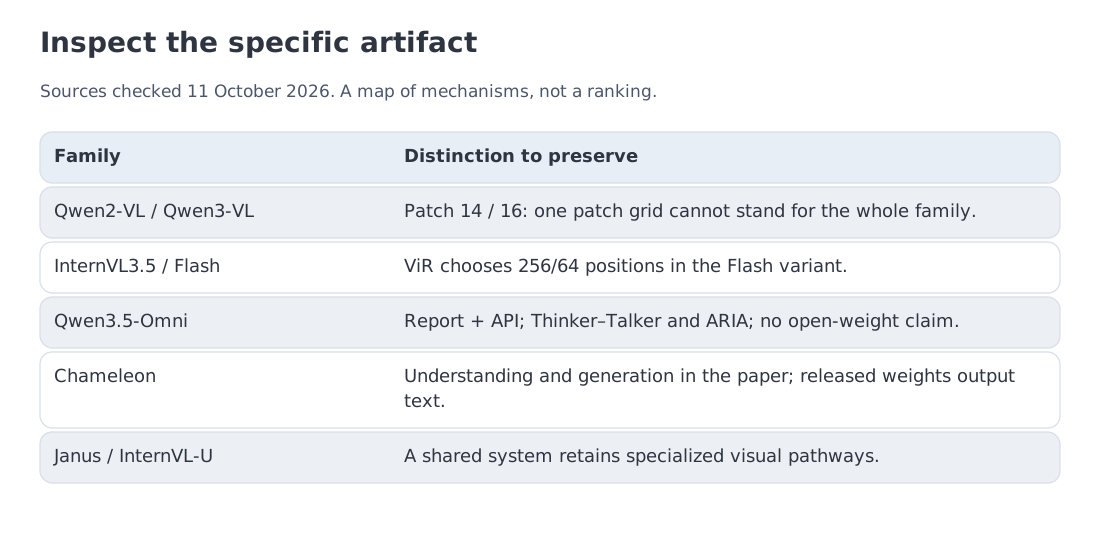 The snapshot compares documented architecture and I/O rather than reconstructing proprietary internals from product behavior.
The table below is not a leaderboard. It is a set of documented answers to the four obligations introduced in Section 1.
| System | Input | Output | Architectural emphasis | Public evidence |
|---|---|---|---|---|
| Qwen3-VL | text, images, video | text | dynamic resolution, interleaved M-RoPE, DeepStack, 256K | report, code, and released model family |
| InternVL3.5 / Flash | text, images, video | text | ViR in Flash, decoupled vision/LLM deployment, Cascade RL | report, code, and weights |
| Qwen3.5-Omni | text, images, audio, video | text and streaming speech | Thinker–Talker, TMRoPE, ARIA, Hybrid-Attention MoE, 256K | report and documented API; not a claim of open weights |
| InternVL-U | text and images | text, image generation, editing | multimodal LLM plus MMDiT generation head | 4B system report |
| Chameleon | text and images | paper: text/images; released weights: text | discrete-token early fusion | paper and family artifacts |
| Janus | text and images | text and images | separate visual pathways, shared Transformer | paper, code, and model family |
This is a mechanism-oriented selection verified on 11 October 2026, not an exhaustive release ranking. Configuration still matters within a family: Qwen3-VL uses 16-pixel patches, whereas our 1008×1008, patch-14 example uses Qwen2-VL-like geometry. The Qwen3.5-Omni report's “256K” training stage specifies 262,144 positions. The 256,000-position classroom calculation is a separate scenario.
The first axis is input-budget control. Qwen3-VL combines dynamic processing, interleaved M-RoPE, DeepStack, and a 256K context. InternVL3.5-Flash uses ViR and decoupled placement of the vision encoder and LLM. Both produce text, but one emphasizes a common interleaved sequence while the other exposes a stronger routing and deployment boundary.
The second axis is the output contract. Qwen3.5-Omni must produce streaming speech, so Thinker–Talker, TMRoPE, and ARIA are part of its architecture passport. The report gives different limits for different signals—more than ten hours of audio and 400 seconds of 720p video at one frame per second. Those limits follow from a concrete processor and architecture, not from the 256K context number alone.
The third axis is the location of specialization. Chameleon shares discrete tokens, Janus shares the Transformer while separating visual pathways, and InternVL-U shares language-centered reasoning while delegating image rendering to an MMDiT head. Similar external capabilities arise from different internal boundaries.
This is the chapter’s argument in compact form. Multimodal systems differ in where they compress evidence, where they preserve structure, and where they specialize output. For a proprietary API, the defensible record is limited to documented inputs, outputs, limits, pricing, and date. Interface behavior alone cannot reveal whether the service contains one end-to-end model or a coordinated cascade.
17. Follow one request through a multimodal passport
A useful passport begins with an actual media request rather than a model name. Follow the evidence through five stages.
1. Identify the input-processing pipeline
Record how raw media becomes positions:
patch_size,temporal_patch_size, andspatial_merge_size;- pixel bounds and rounding rules;
- tiling and thumbnail policy;
- video frame sampling;
- audio sample rate, encoder stride, and positions per second.
These fields convert pixels and seconds into a token budget. A maximum context length without them says little about usable multimedia capacity.
2. Trace the fusion path
Determine whether visual vectors enter decoder self-attention, are reduced by a resampler, or remain in external memory accessed through cross-attention. Record whether vision and language are jointly trained, whether understanding and generation use separate pathways, and whether output modalities have dedicated decoders.
This stage decides whether ordinary decoder-KV arithmetic applies.
3. Trace the output path
Input support does not imply output generation. Identify which module emits text, image latents, audio-codec tokens, or waveform chunks, and at what rate.
4. Measure the system on the real request
Collect:
- visual or audio positions after preprocessing;
- encoder latency;
- language prefill time;
- KV and peak memory;
- time to first text token (TTFT), inter-token latency (ITL), or first-audio latency;
- reuse when several questions refer to the same media object.
The result shows not merely whether the request fits, but which component is the bottleneck.
5. Record artifact status
Distinguish paper, source code, open weights, hosted API, and product demonstration. They support different levels of inspection and reproduction. A behavioral test can verify an exposed capability, but not internal topology: an API may route between specialized models, or a product may disable a generation head that exists in the underlying system.
The completed passport answers the chapter’s opening question. It shows how physical evidence became a model representation, how much it cost, which structure survived, and which component produced the output.
20. Key takeaways and sources
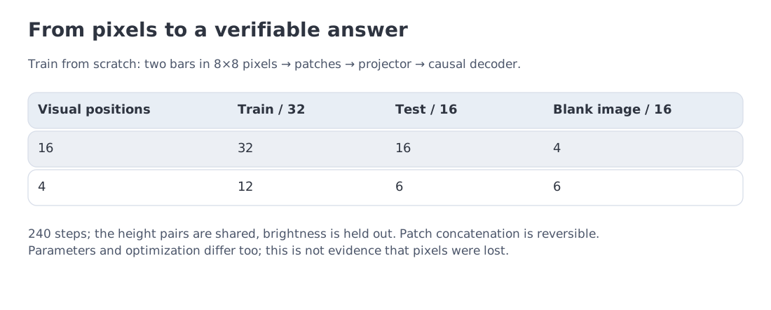 A complete trainable pixels-to-answer path. The 16- and 4-position configurations achieve 16/16 and 6/16 on held-out brightness; blank-image controls achieve 4/16 and 6/16. These are teaching-model results, not a large-VLM benchmark.
The chapter began with one media-rich request and four design obligations. Most architectural differences can now be read as different placements of those obligations.
Representation. CLIP and SigLIP create semantic alignment. ViT converts image area into patch positions. Audio encoders and codecs do the same for a temporal signal. The representation decides what evidence reaches language-level reasoning.
Budget. The declared examples produce 576, 2,880, and 1,296 visual positions. Under the 32-layer GQA self-attention contract, they create 72, 360, and 162 MiB of KV state. A different fusion topology requires a different accounting model.
Compression and connection. An MLP changes width but keeps positions. A Q-Former or resampler reduces position count through an information bottleneck. Cross-attention keeps visual state outside the text stream. A connector moves cost between components; it does not erase it.
Structure. Dynamic resolution makes compute depend on the input. M-RoPE-style schemes preserve height, width, and time. Video turns context length into evidence selection: 7,200 frames at 576 tokens each produce 4.15 million positions before text.
Output. Chameleon, Janus, and InternVL-U show that one user interface does not require one visual representation. Thinker–Talker shows the same for speech: evidence integration and audio generation may share training and context while operating with different clocks.
Engineering conclusion. A “vision/audio/video supported” label is not a system specification. We need the processor, token geometry, fusion path, state layout, output decoder, measurements, and artifact status.
Primary sources
- ViT — An Image is Worth 16×16 Words
- CLIP — Learning Transferable Visual Models From Natural Language Supervision
- SigLIP — Sigmoid Loss for Language Image Pre-Training
- Flamingo — a Visual Language Model for Few-Shot Learning
- BLIP-2 — Bootstrapping Language-Image Pre-training
- LLaVA — Visual Instruction Tuning
- LLaVA-1.5 — Improved Baselines with Visual Instruction Tuning
- Qwen2-VL — Dynamic Resolution and M-RoPE
- Qwen2.5-VL — technical report
- Qwen3-VL — technical report
- InternVL3.5 — technical report
- Chameleon — Mixed-Modal Early-Fusion Foundation Models
- Janus — Decoupling Visual Encoding for Understanding and Generation
- InternVL-U — Understanding, Reasoning, Generation and Editing
- Qwen2.5-Omni — technical report
- Qwen3.5-Omni — technical report
- Chameleon — released interface documentation
- Qwen3-VL — developer code and processor instructions
- SigLIP — reference loss implementation
- Step-Audio 2 — technical report
Next: Module 17 turns to embeddings, retrieval, and RAG. The contrastive geometry from Section 5 becomes a mechanism for searching external data.
Landscape verified: 11 October 2026. Patch counts, KV state, InfoNCE, dense-equivalent training, and video budget are reproducible module scenarios; a real processor may add resizing, padding, temporal patches, and separator tokens.