Module 6. Normalization, activations, and the anatomy of a Transformer block
Modern LLMs · revised October 11, 2026
Attention lets tokens exchange information. To turn it into a useful block, we also need a state that persists between layers, a way to control numerical scale, and a network that transforms each token's features. This module puts those pieces together and accounts for their parameters.
Before you start. You need projections and residual connections from M3, and attention heads and GQA from M5. Equations use column vectors; NumPy stores tokens as rows, so projection matrices multiply on the right.
Reading routes
- First pass: §1 → §§4–10, skipping expandable implementations → §§14–15 → §20. Check Q1–Q6 in §18 and E1–E3 in §19; Q7 and E7 depend on the mHC discussion in §12 and belong to a return visit. Follow the shapes in §10 to the model total. This route prepares you for M7.
- Second pass: bridges B07/B08 in §§5/9, code in §13, and the notebook. Test reduction axes, near-zero inputs, low precision, and gradients; solve exercises 1–3 and 6–7.
- Reference pass: §§2–3 give history and classical connections; §§11–12 introduce element-wise alternatives and multiple streams; §§16–17 help you inspect real architectures. Projects 4–5 extend the experiments.
1. The three jobs surrounding attention
At each token position, the block receives a state . The model width is the number of features in that state. A residual stream carries it through successive layers. Each residual connection adds a learned update of the same shape: .
Attention reads across positions. The feed-forward network (FFN) transforms each position separately, sharing its weights across tokens. Normalization controls the scale at which these operations read or write features. Neither an FFN nor a normalizer moves a token to a different position.
We measure scale using the root mean square:
The vector has mean zero but RMS one. Squaring prevents opposite signs from hiding the size of the coordinates.
Three questions guide the module: what transformation does a norm perform, where does it sit relative to residual addition, and what does a gated FFN cost? A four-coordinate example, a 36-step linear stack, and the Llama-3.1-8B parameter ledger will make the answers concrete.
2. How the block evolved
This historical section is optional on a first reading. The equations for the named designs follow in §§5–12.
LayerNorm (2016) normalized an example's features without collecting batch statistics. The original Transformer placed it after the residual addition: Post-LN. Moving it to the sublayer input gives Pre-LN. Xiong et al. connected the resulting initial gradient behavior to learning-rate warmup in their setting. Their findings do not prohibit every Post-LN training run without warmup. Paper.
RMSNorm (2019) removed mean subtraction. Its authors reported comparable quality and runtime reductions of 7–64% across their tested systems. That range is not an estimate for a current decoder: the saving depends on the workload and implementation. RMSNorm.
GLU variants introduced two FFN projections whose outputs multiply. DeepNorm changed residual scaling and initialization for deep networks. Peri-LN places norms on both sides of a sublayer; OLMo2 normalizes its output before addition. DyT and DyISRU investigate element-wise alternatives to feature normalization, while mHC changes connections between residual streams. These choices affect different parts of the graph and can coexist.
3. Three useful classical analogies
LayerNorm resembles per-example standardization, but it is not whitening: it neither estimates a full covariance matrix nor rotates the feature basis. RMSNorm retains only scale control. The preconditioning analogy is therefore local and practical—normalizers keep the numerical range seen by later matrices more predictable.
Residual updates resemble Euler steps:
This viewpoint is useful for asking how large an update is and how errors accumulate with depth. It is not an exact continuous-time model because the functions change from layer to layer and the step size need not be small.
Gated FFNs illustrate a third idea: multiplicative interaction. Two separately learned projections are multiplied element-wise, so the input controls both what is represented and how strongly it passes. Without a nonlinearity, the product of two linear projections would be quadratic in the input. A SiLU gate makes this a nonlinear, input-dependent interaction; its cost includes a third projection. This explains the mechanism without assuming a universal advantage at every width or parameter budget.
4. A block makes two successive residual updates
In Pre-LN, attention reads a normalized state. The FFN then reads the state after the attention update:
Here identifies the layer, and are its two normalizers. Attention and FFN are sequential branches, not two independent functions of the original .
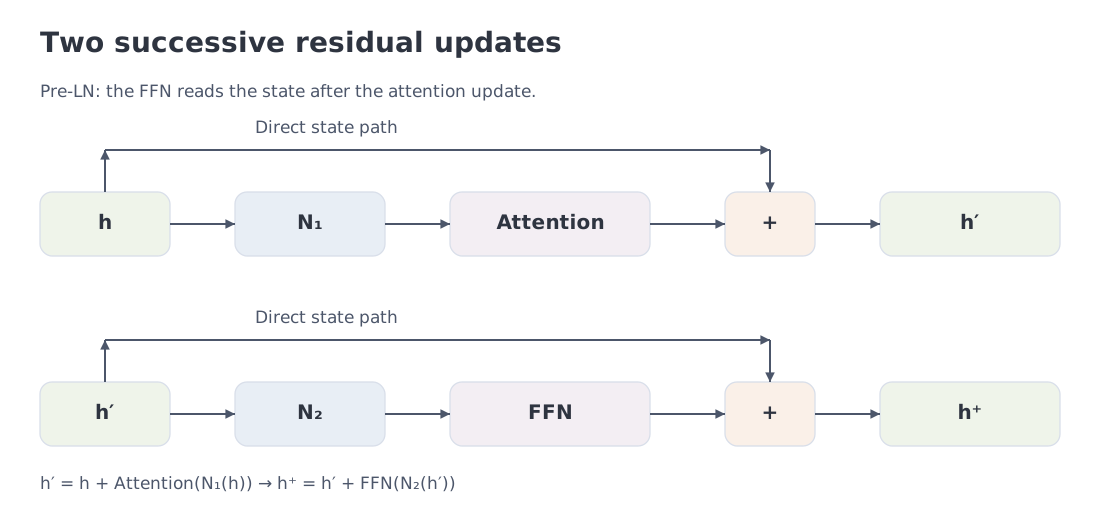 Attention updates the state first; the FFN reads that updated state.
For a vector-valued function, the Jacobian collects all partial derivatives: its entry tells us how output coordinate changes when input coordinate changes. With , this is a matrix. Differentiating a residual step gives , where is the identity matrix and is the branch Jacobian. This direct path is useful, but the sum need not be well conditioned. Taking gives . Nor does a bypass make a trained branch disposable. Removing it changes a learned function and requires a quality check.
5. What LayerNorm and RMSNorm compute
For a token vector , define its feature mean and variance:
Computing one statistic from several coordinates is a reduction. The divisor is , not the sample-variance correction. The two norms are
The learned vectors rescale and shift features; keeps the denominator away from zero. Our RMSNorm definition has a scale and no bias. Both reductions operate on features of one token, not across tokens or the batch.
For , , , and , we have , , and . The outputs are approximately
Before its learned scale, RMSNorm preserves signs and coordinate ratios but does not enforce zero mean. A constant nonzero vector distinguishes the norms: centered LayerNorm returns zero before its affine step, whereas RMSNorm does not.
Epsilon matters near zero
Before multiplication by , the normalization gain is at most . At input RMS it is 707.1 with and 301.5 with . This bounds the multiplier, not all learned output coordinates.
Exact invariance to positive scaling requires and a nonzero vector. With fixed positive epsilon,
Approximate invariance requires both and . A very small positive can violate the second condition even when the original input is large. The notebook includes a near-zero counterexample.
FP16 squaring can overflow or underflow before reduction. Promoting only the mean cannot restore lost information; promote the input before squaring. Our bridge works in at least FP32 and preserves FP64 inputs. A model implementation may choose a different contract: gpt-oss explicitly uses FP32.
Second pass: RMSNorm from NumPy to PyTorch, including gradients
NumPy → PyTorch · B07 — RMSNorm: reduction, dtype, and autograd
Compare finite floating inputs [..., D], D>0, and an optional weight [D], with finite eps>0. API comparisons use a common floating dtype and device for input and weight. Squares, their sum, and the output must fit the working format; merely being finite in FP64 does not ensure this. NumPy exposes the reduction, while PyTorch adds autograd.
import numpy as np
import torch
import torch.nn.functional as F
1. Explicit NumPy implementation
def numpy_rms_norm(x: np.ndarray, weight: np.ndarray | None = None, *, eps: float = 1e-6) -> np.ndarray:
    x = np.asarray(x)
    if x.ndim == 0 or x.shape[-1] == 0 or not np.isfinite(x).all() or not np.isfinite(eps) or eps <= 0:
        raise ValueError("x must be finite and eps positive")
    work = x.astype(np.float64, copy=False)
    y = work / np.sqrt(np.mean(work * work, axis=-1, keepdims=True) + eps)
    if weight is not None:
        w = np.asarray(weight, dtype=np.float64)
        if w.shape != (x.shape[-1],) or not np.isfinite(w).all():
            raise ValueError("weight must be finite with shape [D]")
        y = y * w
    return y.astype(x.dtype, copy=False) if np.issubdtype(x.dtype, np.floating) else y
The NumPy reference exposes the last-dimension mean square, , reciprocal square root, and the learned per-coordinate scale.
2. The same mathematics as explicit PyTorch operations
def torch_rms_norm_explicit(
    x: torch.Tensor,
    weight: torch.Tensor | None = None,
    *,
    eps: float = 1e-6,
) -> torch.Tensor:
    if not x.is_floating_point() or x.ndim == 0 or x.shape[-1] == 0:
        raise ValueError("x must be floating with a nonempty last axis")
    if not np.isfinite(eps) or eps <= 0:
        raise ValueError("eps must be finite and positive")
    work = x.to(torch.float32) if x.dtype in (torch.float16, torch.bfloat16) else x
    rms_inv = torch.rsqrt(work.square().mean(dim=-1, keepdim=True) + eps)
    y = work * rms_inv
    if weight is not None:
        if weight.shape != (x.shape[-1],):
            raise ValueError("weight must have shape [D]")
        y = y * weight.to(work.dtype)
    return y.to(x.dtype)
The explicit path widens FP16/BF16 to FP32 before squaring and restores the input dtype after the gain. FP64 stays FP64 for derivative checks.
3. Optimized or library PyTorch API
def torch_rms_norm(x: torch.Tensor, weight: torch.Tensor | None = None, *, eps: float = 1e-6) -> torch.Tensor:
    return F.rms_norm(x, [x.shape[-1]], weight=weight, eps=eps)
F.rms_norm moves the reduction into a library operator that may use an optimized implementation.
| Aspect | NumPy | PyTorch |
|---|---|---|
| Reduction | np.mean(..., axis=-1) | mean(dim=-1) |
| Reciprocal root | 1 / np.sqrt | torch.rsqrt |
| Weight | broadcast array [D] | learned parameter [D] |
| Accumulation | float64 reference | explicit path: at least FP32; check API separately |
| Gradient | none | checked with gradcheck |
Executable parity and edge-case check
rng = np.random.default_rng(7)
x_np = rng.standard_normal((3, 5)); w_np = rng.standard_normal(5)
np_out = numpy_rms_norm(x_np, w_np, eps=1e-6)
x = torch.tensor(x_np, dtype=torch.float64, requires_grad=True)
w = torch.tensor(w_np, dtype=torch.float64, requires_grad=True)
explicit = torch_rms_norm_explicit(x, w, eps=1e-6)
api = torch_rms_norm(x, w, eps=1e-6)
np.testing.assert_allclose(np_out, explicit.detach().numpy(), rtol=1e-10, atol=1e-10)
torch.testing.assert_close(api, explicit, rtol=1e-10, atol=1e-10)
assert torch.autograd.gradcheck(lambda a, b: torch_rms_norm_explicit(a, b, eps=1e-6), (x, w))
for a, b in zip(torch.autograd.grad(explicit.square().sum(), (x, w)),
                torch.autograd.grad(api.square().sum(), (x, w))):
    torch.testing.assert_close(a, b, rtol=1e-9, atol=1e-10)
for dtype in (torch.float16, torch.bfloat16):
    large = torch.full((2, 8), 1000.0, dtype=dtype)
    torch.testing.assert_close(torch_rms_norm_explicit(large), torch.ones_like(large))
print("B07 explicit NumPy / PyTorch / F.rms_norm: PASS")
Complete executable file: m06_block_bridges.py
Official API: PyTorch rms_norm.
6. Placement changes the computation graph
Let be an attention or FFN sublayer and a normalizer.
| Placement | Residual step | What is normalized? |
|---|---|---|
| Post-LN | The updated state | |
| Pre-LN | The branch input | |
| Peri-LN | Both ends of the branch | |
| OLMo2-style | The branch output only |
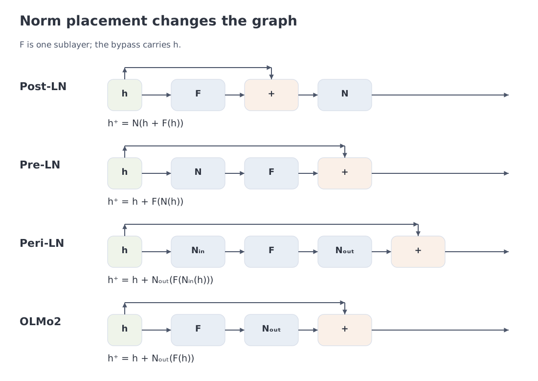 Locate each norm relative to F and the residual addition.
Post-LN has Jacobian , so even the residual path passes through normalization. For Pre-LN, apply the chain rule: . Its complete Jacobian is therefore : the direct identity term remains outside the product. Neither expression guarantees good optimization under every initialization and optimizer.
Peri-LN controls the contribution being added, although learned output scales can change its size. The paper reports experiments up to 3.2B parameters. OLMo2 lacks the paired input norm, so its output-only arrangement should not be labeled Peri-LN. Peri-LN; OLMo2 code.
A controlled forward-scale experiment
Using seed 5, draw the 256 coordinates of independently from a standard normal distribution and generate 36 independent matrices with entries from . Reuse the same input and matrices in three recurrences:
Here . It has no learned scale and uses a denominator floor, rather than additive epsilon. At step 36, RMS is approximately 412,442, 6.423, and 1, respectively.
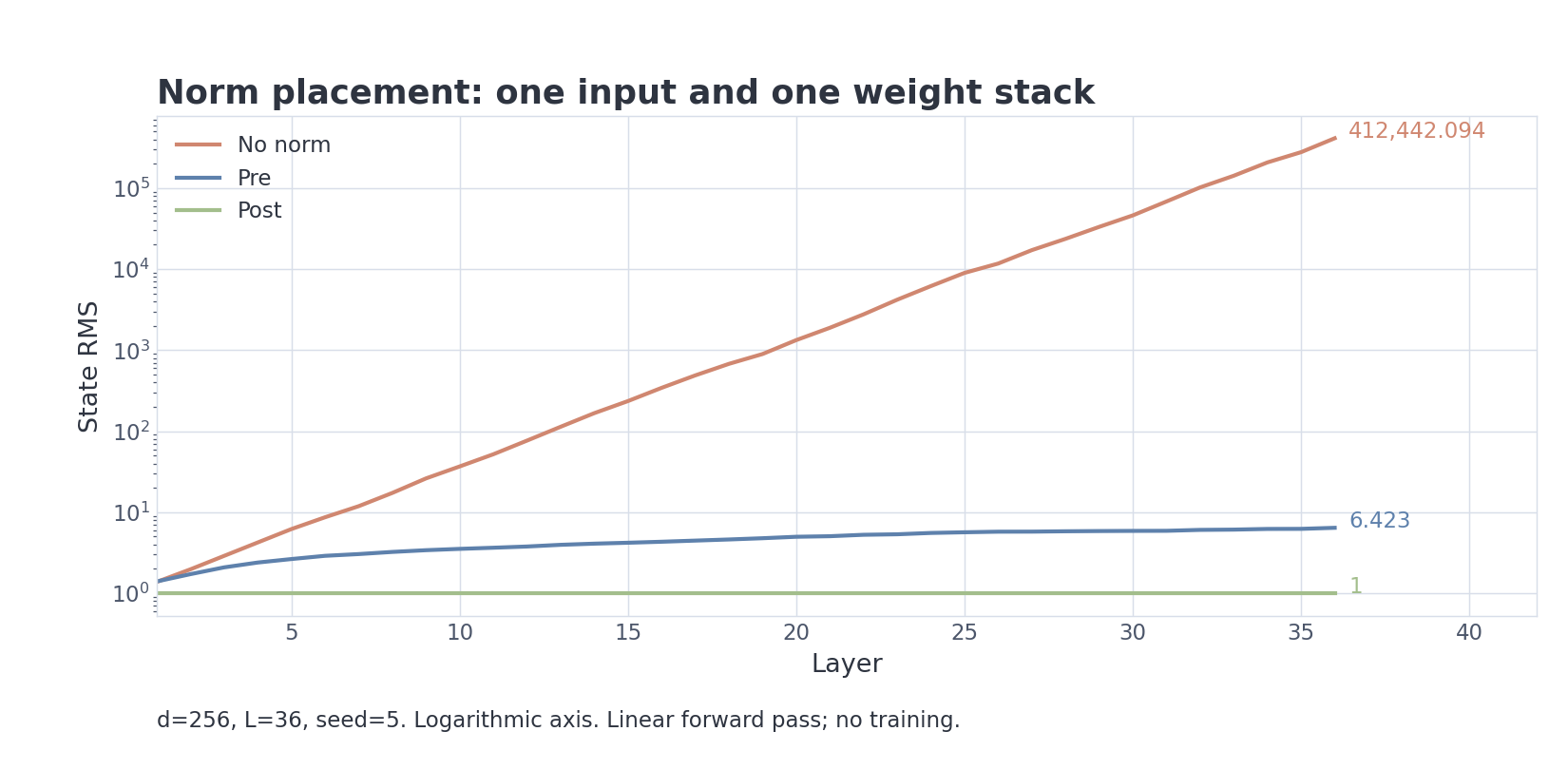 One input and weight stack isolate placement; the vertical axis is logarithmic.
This measures forward scale in a linear residual system. There is no loss or training update. Post has unit RMS by construction; pre still accumulates updates. The notebook also compares Pre-LN and Peri-LN on one frozen attention–FFN stack.
7. Q/K normalization: check the equation and the axis
An attention score is , with head width . Scaling both vectors by scales the score by and can concentrate softmax on very few keys.
Original QKNorm uses L2-normalized vectors and a learned scale :
The scale replaces the usual factor. Practical implementations guard a zero length with a stabilizer. The authors reported an average gain of 0.928 BLEU across five low-resource translation pairs under their protocol. BLEU is a translation metric based on overlap with reference translations; this reported gain concerns that evaluation setting. QKNorm.
Per-head RMSNorm is different. Ignoring epsilon and learned scales, normalized vectors have length . With the usual attention denominator the score becomes , rather than a unit-vector dot product.
The axis also matters. Qwen3 normalizes within each head. OLMo2 normalizes the entire Q projection, and separately the entire K projection, before splitting heads. Changing one head can therefore change other heads' denominators in OLMo2. The notebook demonstrates this with two heads of width two. Qwen3; OLMo2.
Logit soft-capping instead transforms computed scores as for . It bounds scores without normalizing Q or K. Gradient clipping belongs to optimization and does not replace any of these forward operations.
8. Why a gate adds a matrix
A conventional FFN widens a token vector, applies a nonlinearity, and projects back:
The intermediate width is ; biases are omitted here. Removing the nonlinearity would collapse the two matrices into one linear map. Common nonlinearities are
where is the standard-normal cumulative distribution function and . GELU and SiLU suppress negative inputs smoothly instead of zeroing the entire negative half-line.
The approximation has maximum absolute error 0.020335 against exact GELU on 4,001 evenly spaced points in . This is a measured approximation on a specified grid, not equality of functions.
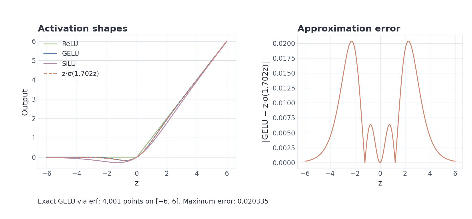 Shared axes compare activations; a separate panel shows the GELU approximation error.
A gated FFN learns two projections, and , then multiplies their transformed outputs coordinate by coordinate. SwiGLU is
Here means element-wise multiplication. Although the gate depends on the input, is not a probability or a value restricted to . The third matrix restores width for residual addition. ReGLU and GEGLU use ReLU and GELU gates instead; Shazeer compared these variants under matched budgets. GLU Variants.
9. Budgeting SwiGLU and reading its variants
Two bias-free FFN matrices cost parameters; SwiGLU costs . Matching a conventional FFN of width gives
Real models may choose another width or round it for implementation reasons. is a budget match, not part of SwiGLU's definition.
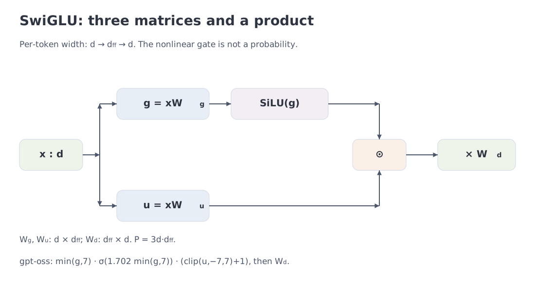 The gate projection passes through SiLU, multiplies the up branch, then feeds the down projection.
The gpt-oss reference uses a specific variant:
Only the upper gate tail is clamped; the up branch is clamped at both ends. This defines the checkpoint's activation. Its training motivation cannot be established from a function body alone. Pinned implementation.
For the diagnostic slice , the product before the down projection is:
| -9 | 0.000012019 |
| -2 | 0.064341377 |
| 0 | 0 |
| 2 | 5.806975869 |
| 7 | 55.999625026 |
| 9 | 55.999625026 |
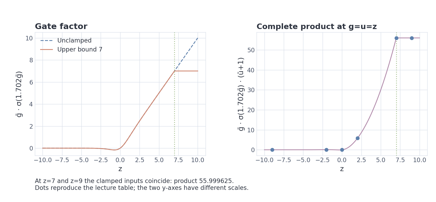 On this slice the gate factor saturates near 7; the complete product approaches 56.
A gate-factor curve alone cannot reproduce the product table. At , a small negative gate factor multiplies , giving a small positive product. At 7 and 9 the two clamped inputs coincide exactly.
Second pass: stable activation code and gradient checks
NumPy → PyTorch · B08 — SwiGLU and a bounded variant
Both implementations keep the gate and up branches explicit. alpha, optional clipping, and the up-branch shift are visible parameters.
import numpy as np
import torch
1. Explicit NumPy implementation
def numpy_swiglu(
    gate: np.ndarray,
    up: np.ndarray,
    *,
    alpha: float = 1.0,
    gate_limit: float | None = None,
    up_limit: float | None = None,
    shift_up: float = 0.0,
) -> np.ndarray:
    gate, up = np.asarray(gate), np.asarray(up)
    if gate.shape != up.shape or not np.isfinite(gate).all() or not np.isfinite(up).all():
        raise ValueError("gate and up must be finite arrays of the same shape")
    if not np.isfinite(alpha) or not np.isfinite(shift_up):
        raise ValueError("alpha and shift_up must be finite")
    if any(v is not None and (not np.isfinite(v) or v <= 0) for v in (gate_limit, up_limit)):
        raise ValueError("limits must be finite and positive")
    g = gate.astype(np.float64, copy=False)
    u = up.astype(np.float64, copy=False)
    if gate_limit is not None:
        g = np.minimum(g, gate_limit)
    if up_limit is not None:
        u = np.clip(u, -up_limit, up_limit)
    sigmoid = np.exp(-np.logaddexp(0.0, -alpha * g))
    y = g * sigmoid * (u + shift_up)
    dtype = np.result_type(gate.dtype, up.dtype)
    return y.astype(dtype, copy=False) if np.issubdtype(dtype, np.floating) else y
Both branches remain visible: the gate passes through a SiLU-like nonlinearity and multiplies the up branch. alpha, clipping, and the shift are explicit parameters.
2. The same mathematics as explicit PyTorch operations
def torch_swiglu(
    gate: torch.Tensor,
    up: torch.Tensor,
    *,
    alpha: float = 1.0,
    gate_limit: float | None = None,
    up_limit: float | None = None,
    shift_up: float = 0.0,
) -> torch.Tensor:
    if gate.shape != up.shape:
        raise ValueError("gate and up must have the same shape")
    if gate.dtype != up.dtype or not gate.is_floating_point() or gate.device != up.device:
        raise ValueError("gate and up must share a floating dtype and device")
    if not np.isfinite(alpha) or not np.isfinite(shift_up):
        raise ValueError("alpha and shift_up must be finite")
    if any(v is not None and (not np.isfinite(v) or v <= 0) for v in (gate_limit, up_limit)):
        raise ValueError("limits must be finite and positive")
    dtype = torch.float32 if gate.dtype in (torch.float16, torch.bfloat16) else gate.dtype
    g, u = gate.to(dtype), up.to(dtype)
    if gate_limit is not None:
        g = g.clamp(max=gate_limit)
    if up_limit is not None:
        u = u.clamp(min=-up_limit, max=up_limit)
    return (g * torch.sigmoid(alpha * g) * (u + shift_up)).to(gate.dtype)
NumPy uses logaddexp for a stable sigmoid; PyTorch uses torch.sigmoid, retains autograd, and widens half-precision intermediates. Clamp has no ordinary derivative at its kinks, so finite-difference checks use points on either side.
| Aspect | NumPy | PyTorch |
|---|---|---|
| Nonlinearity | explicit sigmoid | torch.sigmoid |
| Gate bound | np.minimum | Tensor.clamp(max=...) |
| Up bound | np.clip | Tensor.clamp(min=..., max=...) |
| Standard SwiGLU | no limits, shift_up=0 | same contract |
| Gradients | none | autograd; clamp kinks are tested separately |
Executable parity and edge-case check
rng = np.random.default_rng(8)
g_np = rng.uniform(-4, 4, (3, 5)); u_np = rng.uniform(-4, 4, (3, 5))
kwargs = dict(alpha=1.702, gate_limit=7.0, up_limit=7.0, shift_up=1.0)
np_out = numpy_swiglu(g_np, u_np, **kwargs)
g = torch.tensor(g_np, dtype=torch.float64, requires_grad=True); u = torch.tensor(u_np, dtype=torch.float64, requires_grad=True)
t_out = torch_swiglu(g, u, **kwargs)
np.testing.assert_allclose(np_out, t_out.detach().numpy(), rtol=1e-10, atol=1e-10)
assert torch.autograd.gradcheck(lambda a, b: torch_swiglu(a, b, **kwargs), (g, u))
extreme = np.array([-1000., -9., 0., 9., 1000.])
with np.errstate(over='raise', invalid='raise'):
    stable = numpy_swiglu(extreme, np.ones_like(extreme), **kwargs)
np.testing.assert_allclose(stable, torch_swiglu(torch.tensor(extreme), torch.ones(5, dtype=torch.float64), **kwargs))
outside = torch.tensor([-9., 9.], dtype=torch.float64, requires_grad=True)
assert torch.autograd.gradcheck(lambda a: torch_swiglu(a, a, **kwargs), (outside,))
print("B08 forward + gradient: PASS")
Complete executable file: m06_block_bridges.py
10. From tensor shapes to 8,030,261,248 parameters
Take , , 32 layers, , 32 query heads, 8 KV heads, and head dimension 128. The model is bias-free and uses separate input and output embeddings.
Q and O each have entries; K and V each have . In general,
The Llama 3 report lists the principal dimensions and rounds the vocabulary to 128K. The exact above is part of our frozen counting contract. Report, Table 3.
With this geometry the attention matrices cost
The SwiGLU matrices cost
Two RMSNorm scales add . Therefore
but the complete block is
With two embedding tables and one final norm:
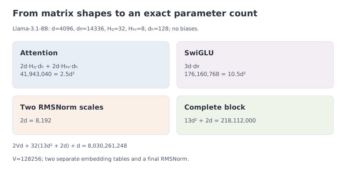 The matrix estimate and the exact block are shown separately.
The FFN accounts for about 80.8% of the full block. The final term is the last RMSNorm scale. Small norm vectors still belong in an exact parameter count.
Activations, masks, caches, and rotary buffers are not learned parameters in this ledger. Tying the input and output weights would replace by . The notebook checks the formula against a small block's actual arrays. The repository validator also sums the 8B geometry as PyTorch meta tensors without allocating its weights.
11. Element-wise alternatives: DyT and DyISRU
On the reference route, we can ask whether the feature reduction itself is necessary. Dynamic Tanh (DyT) computes
with a learned scalar and feature vectors . It has no shared denominator: a coordinate's output is independent of neighboring coordinates. The paper reports competitive results in several vision and language settings. DyT.
For the construction behind DyISRU, set aside epsilon and affine parameters and write RMS normalization as
Replace the sum over other coordinates by a positive learned parameter and absorb into the scale:
This is the paper's decoupled construction, not equality to vector RMSNorm on arbitrary inputs. One way to learn a positive is to optimize an unconstrained scalar and set . This function is positive for every finite real in exact arithmetic. The notebook uses a stable library implementation and adds a small floor for finite precision. DyISRU analysis, version 4.
With unit gain and zero bias, the slopes at zero are for DyT and for DyISRU. Choosing and matches those slopes. It does not transfer a fitted coefficient from one function to another.
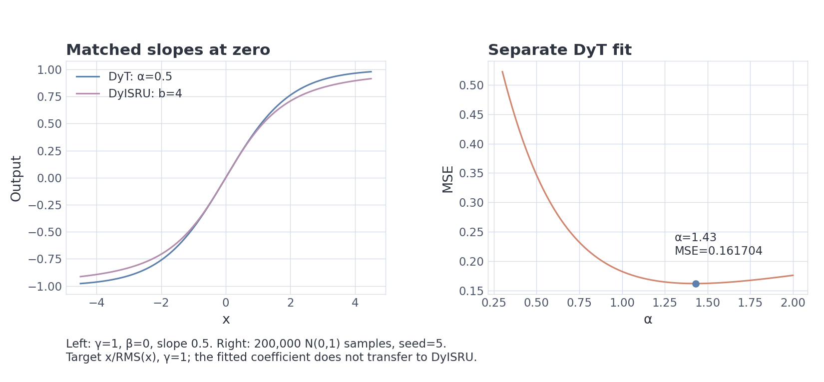 Matched slopes compare shapes; the separate scalar fit has its own objective.
Separately, draw 200,000 standard-normal values with seed 5 and fit to . The grid has 171 coefficients from 0.3 to 2.0; gain stays one and bias zero. Its best point is , with MSE 0.161704. This is a teaching approximation, not a paper-reported constant or a trained Transformer result.
A later study of 1B models over 1,000 steps found a strong adverse interaction between Dynamic Erf and Muon; DyT did not show the same penalty. This limited experiment motivates checking optimizer and activation together rather than establishing a universal ranking. Study.
12. Several residual streams: what mHC constrains
Hyper-Connections carry streams. Put their states in the rows of ; a residual matrix mixes them as . Separate maps combine streams before a sublayer and distribute its output afterward.
Manifold-Constrained Hyper-Connections (mHC) constrain the residual matrix to be doubly stochastic:
This set is the Birkhoff polytope. Each output row is a convex combination of input rows. For a fixed exact matrix, each feature stays between the smallest and largest input-stream values. That does not preserve every stream:
Sinkhorn iterations alternate row and column normalization of a positive matrix. Their limit is doubly stochastic under suitable conditions; a finite result is approximate. The paper uses 20 iterations. Our log-domain exercise compares 1, 20, and 100 and measures both sum residuals. It illustrates constrained mixing, not a complete mHC layer. mHC.
The constraint applies to connections, not to a low-dimensional manifold of hidden states. If depends on , the full derivative includes the derivative of ; a fixed-matrix bound alone does not bound that Jacobian. The pre/post mixing maps have their own parameterizations and are not all doubly stochastic.
DeepSeek-V4 is a public model example. Peri-LN controls branch contributions in an ordinary residual graph; mHC changes how several streams connect around the branch. Model card.
13. A small implementation to inspect
On a second pass, follow an input matrix x[T, d] through this listing. The gate and up matrices have shape [d, d_ff], and the down matrix has shape [d_ff, d]. Because tokens are stored as rows, these arrays are transposes of the column-vector matrices in §9.
RMSNorm promotes low-precision values before squaring, and the sigmoid is evaluated in a stable form. The two FFN functions differ only in the activation between the projections: ordinary SwiGLU or the clamped gpt-oss variant. PreNormStep receives an attention function that must return the input shape; the notebook supplies the full GQA implementation.
Second pass: RMSNorm, two FFNs, and sequential residual updates
import math
import numpy as np

def _floating_array(x: np.ndarray) -> np.ndarray:
    """Validate and return a floating NumPy array without changing its shape."""

    array = np.asarray(x)
    if not np.issubdtype(array.dtype, np.floating):
        raise TypeError("normalization expects a floating-point array")
    if array.ndim == 0 or array.shape[-1] == 0:
        raise ValueError("the normalized last axis must be non-empty")
    if not np.isfinite(array).all():
        raise ValueError("inputs must be finite")
    return array

def _statistics_dtype(dtype: np.dtype) -> np.dtype:
    """Use at least float32 for reductions while preserving float64 inputs."""

    return np.dtype(np.float32) if np.dtype(dtype).itemsize < 4 else np.dtype(dtype)

def rms_norm(
    x: np.ndarray,
    gamma: np.ndarray | float = 1.0,
    eps: float = 1e-6,
) -> np.ndarray:
    """RMS-normalize `[..., d_model]` over the last axis and preserve dtype."""

    if eps <= 0 or not math.isfinite(eps):
        raise ValueError("eps must be finite and positive")
    array = _floating_array(x)
    work_dtype = _statistics_dtype(array.dtype)
    work = array.astype(work_dtype, copy=False)
    mean_square = np.mean(work * work, axis=-1, keepdims=True)
    result = work / np.sqrt(mean_square + eps)
    if np.shape(gamma) not in ((), (array.shape[-1],)) or not np.isfinite(gamma).all():
        raise ValueError("gamma must be a finite scalar or [D] vector")
    result = result * np.asarray(gamma, dtype=work_dtype)
    return result.astype(array.dtype, copy=False)

def stable_sigmoid(x: np.ndarray | float) -> np.ndarray:
    """Compute sigmoid without `exp` overflow on large negative inputs."""

    z = np.asarray(x, dtype=np.float64)
    return np.exp(-np.logaddexp(0.0, -z))

def silu(x: np.ndarray | float) -> np.ndarray:
    """Return SiLU/Swish: x * sigmoid(x)."""

    z = np.asarray(x, dtype=np.float64)
    return z * stable_sigmoid(z)

def gpt_oss_swiglu(
    gate: np.ndarray | float,
    up: np.ndarray | float,
    *,
    alpha: float = 1.702,
    limit: float = 7.0,
) -> np.ndarray:
    """Apply the public gpt-oss gate clamp, up clamp, and `(up + 1)` shift."""

    if limit <= 0 or not math.isfinite(limit):
        raise ValueError("limit must be finite and positive")
    if not math.isfinite(alpha):
        raise ValueError("alpha must be finite")
    g = np.minimum(np.asarray(gate, dtype=np.float64), limit)
    u = np.clip(np.asarray(up, dtype=np.float64), -limit, limit)
    return g * stable_sigmoid(alpha * g) * (u + 1.0)

def swiglu_mlp(x, w_gate, w_up, w_down):
    """Row-vector SwiGLU: two projections, product, then output projection."""
    return (silu(x @ w_gate) * (x @ w_up)) @ w_down

def swiglu_oss_mlp(x, w_gate, w_up, w_down, alpha=1.702, limit=7.0):
    """Apply the gpt-oss activation before the down projection."""
    return gpt_oss_swiglu(x @ w_gate, x @ w_up, alpha=alpha, limit=limit) @ w_down

class PreNormStep:
    """Inspect two sequential residual updates; attention accepts a mask."""
    def __init__(self, norm1, norm2, attention, ffn):
        self.norm1, self.norm2 = norm1, norm2
        self.attention, self.ffn = attention, ffn

    def __call__(self, x, mask):
        h = x + self.attention(self.norm1(x), mask)
        return h + self.ffn(self.norm2(h))
PreNormStep accepts attention as a function with an explicit mask. The notebook supplies GQA and tests causality. This small block isolates normalization and FFN mechanics; positional encoding and a KV cache are outside the experiment.
15. Reading gpt-oss from code rather than from a guessed config field
The pinned reference makes three design choices visible.
First, RMSNorm converts inputs to FP32 before squaring, uses , and returns the original dtype. Second, swiglu implements the 1.702 coefficient, asymmetric gate/up clamps, and the value shift. Third, both attention and MLP use Pre-LN residual updates.
The model configuration exposes sizes, experts, top-k, and the clamp limit. This original schema has no hidden_act field; a converted library schema may have one. The executed function remains the activation contract.
{
  "hidden_size": 2880,
  "intermediate_size": 2880,
  "num_experts": 128,
  "experts_per_token": 4,
  "swiglu_limit": 7.0
}
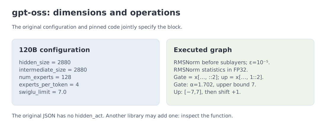 Configuration fields on one side, code-defined behavior on the other.
The intermediate width describes one expert. Total and active parameter accounting therefore depends on routing and belongs in Module 7.
The packed expert projection is interleaved: x[..., ::2] supplies the gate and x[..., 1::2] supplies the up values. Splitting into contiguous halves preserves shapes but changes the function. The repository validator compares our RMSNorm and packed activation against these two functions in the pinned source.
The source manifest records revisions and hashes; M6 stores the original configuration. Dimensions and operations must be read together.
16. A block reference table, as of October 10, 2026
This is a guide to reading open implementations, not an exhaustive model catalog. Expert branches are separate FFNs selected for a token; M7 explains the routing mechanism. A family name never replaces checkpoint flags. The inspected revision and hashes are in the source manifest.
| Family | Block normalization | FFN | Q/K or score treatment |
|---|---|---|---|
| Llama 3.x | Pre-LN RMSNorm | SwiGLU | No separate Q/K norm in inspected code |
| Llama 4 | Pre-LN RMSNorm | Gated dense/expert branches | L2 Q/K on RoPE layers when use_qk_norm is enabled |
| Gemma 2 | RMSNorm at sublayer inputs and outputs | Gated GELU-tanh | Configured attention-logit soft-cap |
| Gemma 3 | RMSNorm at sublayer inputs and outputs | Gated GELU-tanh | Per-head Q/K RMSNorm; soft-cap follows config |
| Gemma 4 text | Input/output RMSNorm plus norms in optional branches | Gated dense/expert branches | Per-head Q/K norms on corresponding projection paths |
| OLMo2 | Post-sublayer RMSNorm before addition | SiLU-gated MLP | Whole Q/K projection RMSNorm before head splitting |
| gpt-oss | Pre-LN RMSNorm | Clamped SwiGLU with | Learned sinks; no Q/K norm in reference |
| DeepSeek-V4 | Sublayer norms and mHC residual mixing | Clamped expert FFN | Depends on attention path |
| Qwen3 | Pre-LN RMSNorm | SiLU-gated MLP | RMSNorm within each Q/K head |
Inspect placement, reduction axis, FFN function, and optional flags in that order. Then verify dimensions and parameter sharing. Unpublished architecture details of a closed model should remain unspecified.
17. Applying the method to vision blocks
A vision Transformer also has norms, attention, an MLP, and residual additions. Its ledger follows from matrix shapes, intermediate width, and bias policy. An encoder may use a noncausal mask, so the language decoder's mask should not be copied automatically.
QKNorm was introduced for low-resource translation in 2020. ViT-22B later used Q/K normalization at large vision scale. These are related applications, not evidence of one universal formula. QKNorm; ViT-22B.
Multimodal configurations frequently separate text and vision towers. Read each independently: activations, epsilon, widths, and placement may differ even within one checkpoint.
20. A practical order for reading an unfamiliar block
 Trace the residual graph, locate the norms, inspect the FFN, then count parameters.
Start with the residual additions: identify the tensors and check their shapes. Locate every norm and record its axis, affine parameters, and working dtype. Follow both gate branches through their product to the output projection. Finally, sum entries in each distinct learned tensor.
These steps explain where information flows, how its scale changes, what transformation is learned, and how many parameters it costs. For the Llama-3.1-8B geometry, each block has matrix entries and another in norms. M7 extends this accounting to routed experts.
On a reference pass, add two distinctions. DyT/DyISRU replace a shared feature statistic with element-wise functions. mHC changes connections between several residual streams. Assess their claims and experiments at those respective levels.
21. primary sources
Primary sources:
- Ba, Kiros, Hinton, Layer Normalization
- Zhang and Sennrich, Root Mean Square Layer Normalization
- Xiong et al., On Layer Normalization in the Transformer Architecture
- Wang et al., DeepNet
- Kim et al., Peri-LN
- Henry et al., Query-Key Normalization
- Shazeer, GLU Variants Improve Transformer
- Zhu et al., Transformers without Normalization
- Stollenwerk, Layer Normalization and Dynamic Activation Functions
- Xie et al., Manifold-Constrained Hyper-Connections
- OpenAI gpt-oss reference implementation
- Hugging Face documentation for OLMo2, Llama 4, Gemma 2, Gemma 3, Qwen3, and DeepSeek-V4
- Official Transformers implementations for OLMo2, Llama 4, Gemma 3, and Qwen3
Next: Module 7 turns the narrow gpt-oss expert into a full Mixture-of-Experts calculation: total versus active parameters, routing, and load balancing.
Sources checked October 10, 2026. Numerical examples use the module-owned fixture; empirical findings retain their source conditions.