Module 20. The complete LLM: from tokens to training and generation

Modern LLMs · additional synthesis module · revision 2026.10.31

By this point, we have studied language models through several different lenses. Attention explained communication between positions; optimization explained how weights change; inference introduced state and token selection; evaluation asked whether the resulting behavior was useful. It is time to put those views together. What, exactly, lies between a token ID and the probability of its continuation? Which parts of that computation learn, and which parts merely organize its execution?

We will construct a complete mathematical description of a particular MiniLLM configuration: a dense autoregressive decoder with pre-RMSNorm, RoPE, GQA, and SwiGLU. Once the construction is explicit, we can identify the operator replaced by MoE, the state carried by an SSM, and the different generation process used by a diffusion model. The final equation will be compact because its components have been explained, rather than because important work has been hidden inside a symbol.

Reading routes

For a first reading, you need matrix multiplication, conditional probability, and the meaning of a gradient. Module 3 provides a refresher; Modules 4–6 develop positions, attention, and the Transformer block. Read Sections 1–10, then 13–14 and 17–20. On this pass, Sections 11–12 can be read for the connection between prediction error and changing weights. Complete Exercises 1–3 and 6 in Section 18; the required material is included in this route.

1. Three computations that should not be conflated

Hold the weights fixed and supply a sequence of known token IDs. The model returns a probability vector for the next token. This is a forward pass. It neither selects a continuation nor updates a parameter.

Training supplies a target continuation, evaluates a loss, and uses its derivatives to update the weights. Generation selects a token, appends it to the context, and repeats the forward pass. The selected token may come from the model's distribution or from a modified decoding distribution. A complete account needs all three computations: a distribution alone is not a training algorithm, and a distribution alone is not yet an answer.

We will omit the batch dimension and follow one example. A batch applies the same operations to several examples and combines the chosen target positions in its loss. Two masks have different jobs throughout: an attention mask controls which context a position can read; a loss mask controls which predictions contribute to learning.

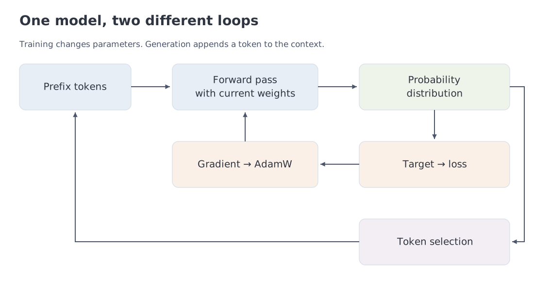
Figure 1. The same probability calculation supports different loops. Training sends derivatives back to parameters; generation sends a selected token back to the input.

2. Notation and the configuration we are describing

Let $x_0=\mathrm{BOS}$ be the beginning-of-sequence token. The continuation $x_1,\ldots,x_N$ includes EOS when the example is intended to represent a completed sequence. To predict $x_t$, the model receives $x_0,\ldots,x_{t-1}$, a prefix of length $t$. Positions are numbered from zero, so row $t-1$ belongs to the last known token, not to the token being predicted.

Our configuration has $h_qd_h=d$, an integer ratio $h_q/h_{kv}$, and even $d_h$. These are assumptions of this derivation, not requirements imposed on every language model. The base model has no linear biases, dropout, QK normalization, attention sinks, or sliding window. RoPE frequencies are not rescaled. Each sequence is a single continuous example; packing independent documents would require additional attention boundaries.

The tokenizer from Module 2 maps text to IDs before this computation begins. Its discrete segmentation algorithm is outside the differentiable forward pass. Our numerical example supplies IDs directly, so the arithmetic does not depend on a corpus snapshot or tokenizer release.

3. Embedding lookup starts the computation

The input representation is a row lookup:

$H^{(0)}=E[x_0,\ldots,x_{t-1}].$

Repeated occurrences of an ID use the same learned row. They will nevertheless acquire different contextual representations, because each position has a different available prefix. It is useful to distinguish the table $E$, which is a parameter, from the selected matrix $H^{(0)}$, which is an activation produced for this input.

Our running example has vocabulary $(\mathrm{BOS},A,B,\mathrm{EOS})$, assigned IDs $(0,1,2,3)$. The complete example is $(0,1,2,3)$: inputs are $(0,1,2)$ and next-token targets are $(1,2,3)$. Choose $V=4$, $d=m=2$, and $L=h_q=h_{kv}=1$. Both the data and the initial weights are synthetic. The four symbols make the arithmetic readable; this is not a model that has learned the meanings of four words.

$E=\begin{bmatrix}1&0\\0&1\\1&1\\-1&0\end{bmatrix},\qquad H^{(0)}=\begin{bmatrix}1&0\\0&1\\1&1\end{bmatrix}.$

There are three input positions and three predictions. The first row receives BOS and predicts A. Keeping this one-position shift explicit prevents a surprisingly easy mistake: training a model to reconstruct the token it has already been given.

4. RMSNorm controls scale before a sublayer

For a row $h$ of width $d$, define

$\rho(h)=\sqrt{\frac1d\sum_{i=1}^{d}h_i^2+\varepsilon},\qquad N_\gamma(h)=\gamma\odot\frac{h}{\rho(h)}.$

We use $\varepsilon=10^{-6}$ to keep the denominator positive. RMSNorm does not subtract the mean, as LayerNorm does. Nor does it normalize to unit Euclidean length: with unit gains and negligible $\varepsilon$, it makes the mean square approximately one.

The operation acts independently on each row, so it does not mix positions or reveal future tokens. There are two distinct gain vectors inside a block, one before attention and one before the FFN, plus a final gain vector after the stack. Equal initial values do not make them shared parameters.

Initialize all three gains to $(1,1)$. The attention input becomes

$X=N_{\gamma_a}(H^{(0)})\approx\begin{bmatrix}1.414212&0\\0&1.414212\\1.000000&1.000000\end{bmatrix}.$

The final row has been rounded for display: both entries are slightly below one because of $\varepsilon$. All later results are computed from full-precision values, not from the rounded matrices printed in the lecture.

5. Projections and RoPE attach a position to a comparison

Attention constructs queries, keys, and values from $X$. For query head $j$ and key/value head $g$,

$Q_j=XW^Q_j,\qquad K_g=XW^K_g,\qquad \mathsf V_g=XW^V_g.$

Each projection has shape $d\times d_h$; its result has shape $t\times d_h$. We reserve plain $V$ for vocabulary size and use $\mathsf V_g$ for value activations. Queries and keys determine the weights of an interaction. Values carry the information that those weights will combine.

RoPE rotates queries and keys at each position. In the rotate_half convention, coordinate $i$ is paired with coordinate $i+d_h/2$, for $i=0,\ldots,d_h/2-1$. With frequency $\omega_i=10000^{-2i/d_h}$ and position $p$, the pair $(a,b)$ becomes

$\begin{aligned}a'&=a\cos(p\omega_i)-b\sin(p\omega_i),\\b'&=a\sin(p\omega_i)+b\cos(p\omega_i).\end{aligned}$

Call this rotation $\mathcal R_p$. Apply it to the rows of $Q_j$ and $K_g$, producing $\widetilde Q_j$ and $\widetilde K_g$. Values are not rotated in this configuration, and the fixed rotation introduces no trainable parameters. The dot product of two rotated vectors depends on their relative rotation, which is how position differences enter the attention score. The coordinate pairing is part of the model definition; changing it without transforming the weights changes the function.

For the example, set $W^Q=W^K=0.5I_2$ and $W^V=\operatorname{diag}(0.5,1)$. There is only one coordinate pair, with $\omega_0=1$, so positions 0, 1, and 2 use angles 0, 1, and 2 radians:

$\widetilde Q=\widetilde K\approx\begin{bmatrix}0.707106&0\\-0.595009&0.382051\\-0.662722&0.246575\end{bmatrix},\quad\mathsf V\approx\begin{bmatrix}0.707106&0\\0&1.414212\\0.500000&1.000000\end{bmatrix}.$

Queries equal keys here only because we chose equal projection matrices. Nothing in the general construction requires that equality.

6. Causal attention and shared key/value heads

GQA lets several query heads read the same key/value head. Number heads from zero and define $g(j)=\lfloor j/(h_q/h_{kv})\rfloor$. Sharing K/V does not average the queries: each head still has its own $W^Q_j$ and can attend differently. The shared projections and their cached activations are where the saving occurs.

Position $i$ may read key position $r$ only when $r\le i$. Encode that condition as an additive mask:

$M_{ir}=\begin{cases}0,&r\le i,\\-\infty,&r\gt i.\end{cases}$

One attention head is now fully specified:

$S_j=\frac{\widetilde Q_j\widetilde K_{g(j)}^\top}{\sqrt{d_h}}+M,\qquad A_j=\operatorname{softmax}_{\rm row}(S_j),\qquad O_j=A_j\mathsf V_{g(j)}.$

The allowed weights in each row sum to one; masked positions have weight zero. Self-attention is allowed, so no row is completely masked in this example. Each output $O_j$ has shape $t\times d_h$. Concatenating heads and multiplying by $W^O\in\mathbb R^{d\times d}$ defines $\mathcal A(X)=\operatorname{Concat}(O_0,\ldots,O_{h_q-1})W^O$.

For the final query in our example, the attention weights are approximately $(0.201972,0.397396,0.400632)$. To see where they come from, consider its score for the first key: $(-0.662722\cdot0.707106+0.246575\cdot0)/\sqrt2\approx-0.331361$. Compute all allowed scores, exponentiate and normalize them, then use the resulting weights to combine the value rows.

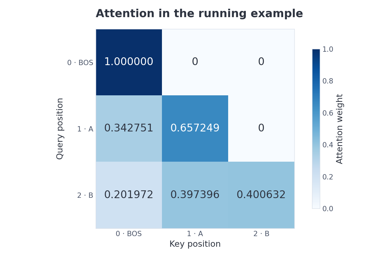
Figure 2. The matrix $A$ for the running example. Entries above the diagonal are zero because of the mask; the remaining entries are computed from queries and keys.

Choose $W^O=0.25I_2$. The first residual addition produces

$Z=H^{(0)}+\mathcal A(X)\approx\begin{bmatrix}1.176777&0\\0.060590&1.232372\\1.085783&1.240658\end{bmatrix}.$

Notice what travels along the residual branch: it is $H^{(0)}$, not its normalized version $X$. The normalization belongs to the attention branch. This distinction matters again when we differentiate the block.

7. SwiGLU completes the block

Attention has exchanged information across positions. The FFN now transforms each position independently. Define

$\mathcal F(Y)=\big[\operatorname{SiLU}(YW^{\rm gate})\odot(YW^{\rm up})\big]W^{\rm down},\qquad\operatorname{SiLU}(a)=a\sigma(a),\quad\sigma(a)=\frac1{1+e^{-a}}.$

The gate and up matrices have shape $d\times m$; the down matrix has shape $m\times d$. Two projections map the representation to $m$ coordinates, the nonlinear branch modulates an elementwise product, and the final projection returns to width $d$. Usually $m$ is larger than $d$; our small examples do not require that choice. This is the SwiGLU construction developed in Module 6.

For our numerical block, use

$W^{\rm gate}=\begin{bmatrix}0.5&-0.25\\0.25&0.5\end{bmatrix},\quad W^{\rm up}=\begin{bmatrix}1&0.5\\-0.5&1\end{bmatrix},\quad W^{\rm down}=0.25I_2.$

The first row of $Y=N_{\gamma_f}(Z)$ is approximately $(1.414213,0)$. Its gate projection is $(0.707106,-0.353553)$ and its up projection is $(1.414213,0.707106)$. Applying SiLU, multiplying the branches, and projecting down gives $(0.167440,-0.025783)$. The negative output is legitimate: SiLU does not discard every negative input.

We can now define a complete block $\mathcal B_\ell$:

$\boxed{\begin{aligned}Z^{(\ell)}&=H^{(\ell-1)}+\mathcal A_\ell\big(N_{\gamma_{a,\ell}}(H^{(\ell-1)})\big),\\H^{(\ell)}&=Z^{(\ell)}+\mathcal F_\ell\big(N_{\gamma_{f,\ell}}(Z^{(\ell)})\big).\end{aligned}}$

Each layer owns separate projections and normalization gains. Our one-layer example ends at

$H^{(1)}\approx\begin{bmatrix}1.344217&-0.025783\\0.023804&1.398300\\1.135097&1.306390\end{bmatrix}.$

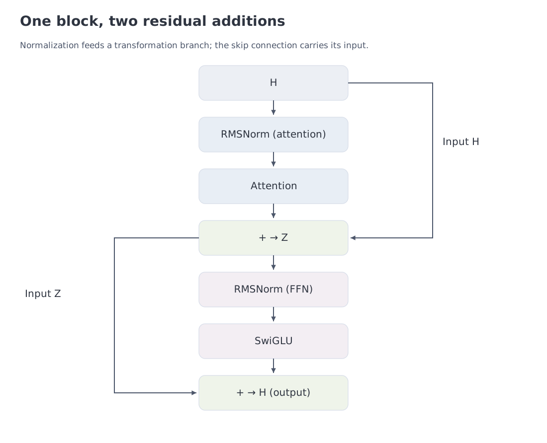
Figure 3. Each normalization feeds a transformation branch. Each skip connection carries the representation from before that sublayer.

8. The stack, output projection, and parameter inventory

Composition applies the rightmost operator first. Stacking the blocks, normalizing their final output, and projecting to the vocabulary gives

$H^{(L)}=(\mathcal B_L\circ\cdots\circ\mathcal B_1)(H^{(0)}),\qquad R=N_{\gamma_o}(H^{(L)}),\qquad\Lambda=RU.$

The entries of $\Lambda$ are logits: unrestricted real scores rather than probabilities. A softmax over the $V$ columns of each row produces the next-token distribution. With tied embeddings, $U=E^\top$. That means one parameter has two computational roles, not two equal copies that an optimizer can update independently. Our base example uses an independent $U$.

A parameter count provides a useful completeness check. For identical dense blocks under the assumptions of Section 2,

$P=n_E Vd+L\big(2d^2+2d h_{kv}d_h+3dm+2d\big)+d,\qquad n_E=\begin{cases}1,&U=E^\top,\\2,&U\text{ is independent.}\end{cases}$

The terms have direct counterparts in the graph. Query and attention-output projections contribute $2d^2$; keys and values contribute $2dh_{kv}d_h$; the three FFN matrices contribute $3dm$. There are $2d$ normalization gains per block and $d$ final gains. Our example has $16+16+12+4+2=50$ parameters. Tying embeddings reduces the count to 42. A second configuration with $d=4,m=3,h_q=2,h_{kv}=1,V=4,L=1$ and independent tables has 128 parameters; using two K/V heads instead gives 144.

Thus $\theta$ includes embedding and output weights, linear projections, and normalization gains. Token IDs, the causal mask, and fixed RoPE frequencies are not learned. Activations, gradients, caches, and optimizer moments occupy memory but are not additional model parameters. The distinction connects this equation to the memory budgets in Modules 9–10.

9. Finish the numerical forward pass

Set the output matrix to

$U=\begin{bmatrix}0&0.5&-0.5&0.25\\0&-0.25&0.5&-0.5\end{bmatrix}.$

Final RMSNorm gives rows of $R$ approximately equal to $(1.413953,-0.027120)$, $(0.024071,1.414008)$, and $(0.927561,1.067535)$. Multiplication by $U$ and a row softmax yield the following results. Every four-entry vector uses the order BOS, A, B, EOS.

The final target receives a relatively low probability. That is not a numerical defect: hand-selected weights have no obligation to predict our sequence well. It gives us a concrete error to follow through training.

The implementation subtracts the largest logit in each row before exponentiation. Adding or subtracting the same constant from every logit leaves softmax unchanged, while unshifted exponentials can overflow. All logarithms here are natural logarithms, so the loss is measured in nats.

10. From a next-token distribution to sequence likelihood and loss

The final row computed on a prefix gives $p_\theta(x_t\mid x_0,\ldots,x_{t-1})$. With a fixed BOS token, the probability of a specified continuation is

$p_\theta(x_1,\ldots,x_N\mid x_0)=\prod_{t=1}^{N}p_\theta(x_t\mid x_0,\ldots,x_{t-1}).$

Include EOS when computing the probability of a completed response. Without EOS, the product describes the probability of the given prefix. During training, the correct sequence is available in advance, so one masked forward pass can calculate all these conditionals. This is teacher forcing: each position receives the correct preceding tokens, not the model's previous guesses. Computing rows in parallel does not grant them access to future positions.

Let $b_t\in\{0,1\}$ select the target positions and let $n=\sum_t b_t\gt0$. The token-averaged cross-entropy is

$\mathcal L(\theta)=-\frac1n\sum_{t=1}^{N}b_t\log p_\theta(x_t\mid x_{\lt t}).$

Here $x_{\lt t}$ includes BOS and all earlier tokens. For a batch, the sum and its denominator cover all selected targets in that batch. Averaging each response first and then averaging responses would assign different weights; the normalization is part of the objective.

In the example, all three targets are selected. Their losses are $0.889986$, $0.742606$, and $1.695530$, giving a mean of 1.109373924. The same value follows directly from the logits through $\log\sum_v e^{\Lambda_{t-1,v}}-\Lambda_{t-1,x_t}$. Selecting only EOS gives a loss of $1.695530$, not one third of that number. If the mask selects nothing, the mean is undefined; the code rejects that case.

11. Backpropagation reaches every learned part

Writing $\nabla_\theta\mathcal L$ is concise, but it should not conceal how the derivative reaches a matrix. Start with one logit row $\lambda$ and target ID $y$. Softmax followed by cross-entropy gives

$\frac{\partial\mathcal L}{\partial\lambda_v}=\frac{b}{n}\big(p_v-\mathbf1[v=y]\big).$

For the final row of our example, this is approximately $(0.082722,0.100724,0.088719,-0.272166)$. The components sum to zero, consistent with the invariance to a common logit shift. The negative derivative of the target logit means that increasing that logit alone would decrease the loss.

Use $G$ to denote an incoming gradient. For a linear operation $Y=XW$, the chain rule gives $G_X=G_YW^\top$ and $G_W=X^\top G_Y$. For a residual operation $Z=H+F(H)$, flattening the arrays into vectors gives $G_H=G_Z+J_F(H)^\top G_Z$. The identity branch provides a direct gradient path; the transformation branch still contributes its own derivative.

For SwiGLU, set $a=YW^{\rm gate}$, $u=YW^{\rm up}$, and $c=\operatorname{SiLU}(a)\odot u$. Then

$G_a=G_c\odot u\odot\big[\sigma(a)+a\sigma(a)(1-\sigma(a))\big],\qquad G_u=G_c\odot\operatorname{SiLU}(a).$

Backpropagate through both projections and add their contributions at $Y$. For RMSNorm on one row, first define $v=G_{N(h)}\odot\gamma$. The derivatives are

$G_h=\frac{v}{\rho}-\frac{h\,(v\cdot h)}{d\rho^3},\qquad G_\gamma=G_{N(h)}\odot\frac{h}{\rho}.$

Sum the gain derivatives over rows. The denominator is the same $\rho$ used in the forward pass, including $\varepsilon$. Dropping that term during differentiation would produce a derivative of a different function.

Attention also decomposes into familiar operations. From $O=A\mathsf V$, obtain $G_A=G_O\mathsf V^\top$ and $G_{\mathsf V}=A^\top G_O$. If $a$ is a row of softmax outputs, its backward pass can be written without materializing a full Jacobian:

$G_s=a\odot\big(G_a-(G_a\cdot a)\mathbf1\big).$

Masked entries have zero derivative. For the allowed scores in $S=\widetilde Q\widetilde K^\top/\sqrt{d_h}+M$,

$G_{\widetilde Q}=G_S\widetilde K/\sqrt{d_h},\qquad G_{\widetilde K}=G_S^\top\widetilde Q/\sqrt{d_h}.$

RoPE sends the derivative through the inverse rotation. Under GQA, contributions from all query heads sharing a K/V head are added. Embedding lookup accumulates gradients into the selected table rows, adding contributions when an ID occurs more than once. If $U=E^\top$, the output projection contributes another gradient to that same table. This accounts for every trainable component listed in Section 8.

The notebook checks the complete path in two ways. PyTorch differentiates its graph automatically; NumPy estimates each of the 50 derivatives through the central difference $(\mathcal L(\theta_i+h)-\mathcal L(\theta_i-h))/(2h)$ with $h=10^{-5}$. A separate run ties embeddings and checks all 42 remaining parameters. This validates the selected smooth configuration in float64, rather than proving correctness for arbitrary architecture changes.

12. AdamW turns derivatives into a new model

A gradient specifies local sensitivity, not a complete update rule. AdamW also needs optimizer state. Let $g_s$ be the gradient on training step $s$. With a global clipping threshold $c$, first compute

$\widetilde g_s=g_s\min\left(1,\frac{c}{\lVert g_s\rVert_2}\right).$

Define the factor as one when the gradient is zero. The norm covers all trainable scalars; this is not independent clipping of each entry. AdamW then updates two moment estimates:

$m_s=\beta_1m_{s-1}+(1-\beta_1)\widetilde g_s,\qquad v_s=\beta_2v_{s-1}+(1-\beta_2)\widetilde g_s^2,$ $\widehat m_s=\frac{m_s}{1-\beta_1^s},\quad\widehat v_s=\frac{v_s}{1-\beta_2^s},\quad\theta_s=(1-\eta_s\lambda)\theta_{s-1}-\eta_s\frac{\widehat m_s}{\sqrt{\widehat v_s}+\varepsilon_{\rm opt}}.$

Squares, square roots, and divisions are elementwise. The learning rate is $\eta_s$; weight decay $\lambda$ may differ between parameter groups. Our experiment assigns $\lambda=0.1$ to matrices and zero to normalization gains. That grouping is an experimental choice, not a universal property of AdamW. Its numerical stabilizer, $\varepsilon_{\rm opt}=10^{-8}$, is separate from the RMSNorm epsilon.

Start with zero moments, $\beta_1=0.9$, $\beta_2=0.95$, $\eta_1=0.01$, and $c=1$. The gradient norm is 0.587186334, so clipping is inactive. Bias correction on the first step gives $\widehat m_1=g_1$ and $\widehat v_1=g_1^2$. After this update, loss on the same sequence falls from 1.109373924 to 1.084831548.

This is a result for one specified step, not a guarantee of monotonic improvement or generalization. Later steps use accumulated moments; repeatedly applying the zero-state first-step formula would not implement AdamW. The notebook compares our update with torch.optim.AdamW and then runs a short training loop that preserves the optimizer state across steps.

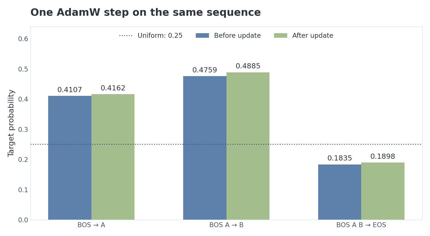
Figure 4. These are the same three predictions from Section 9. The bars show their target probabilities; a uniform distribution over four tokens would assign 0.25.

13. Generation adds a selection rule

At inference time, fix $\theta$ and begin with a known prefix. Greedy decoding selects a maximum-probability token. Sampling instead draws from a distribution, which a decoder may modify. With temperature $\tau\gt0$ and a nonempty candidate set $K$, define

$q(v\mid x_{\lt t})=\frac{\mathbf1[v\in K]\exp(\lambda_v/\tau)}{\sum_{u\in K}\exp(\lambda_u/\tau)}.$

When $\tau=1$ and $K$ is the whole vocabulary, $q=p_\theta$. Top-k keeps the $k$ largest logits and renormalizes over those candidates. Selection, appending, and stopping belong to the generation algorithm. Argmax should be stated as a separate rule, rather than implemented by substituting zero for temperature in this equation.

For the last row of our example, top-2 retains A and B. At $\tau=0.5$, the decoding distribution is $q=(0,0.563116,0.436884,0)$. EOS is excluded on this step even though the base model assigns it probability 0.183502. Consequently, the probability of a sampled continuation under this decoder is a product of its $q$ terms, not the original $p_\theta$ terms.

Append the selected token and compute the next distribution. Stop on EOS or when the specified length limit is reached. Merely including EOS in the vocabulary does not guarantee termination for arbitrary weights and selection rules. A reproducible generation experiment therefore records the weights, initial prefix, decoding settings, and random seed.

14. KV-cache preserves a computation already performed

In this causal architecture, appending a token does not change earlier activations. The argument works layer by layer: normalization and FFN are rowwise, and an earlier attention row gains no newly allowed keys. Keys and values for the processed prefix can therefore be retained.

On a later step, each layer computes Q/K/V only for new positions, appends their K/V to its own cache, and reads all allowed cached keys. Our convention stores rotated keys and unrotated values. Crucially, the new query uses its absolute position: after three processed tokens, the next position is 3, not 0.

For full attention, a single example needs $2Lth_{kv}d_h$ cached scalar values after $t$ tokens. Our one-layer example stores 12 scalars after the three inputs, or 48 bytes in float32 before runtime overhead. The model weights are separate from this count. GQA reduces the number of cached heads to $h_{kv}$ while retaining $h_q$ query heads.

A cache is valid for the same prefix, weights, and positional rules. Updating the weights invalidates it. Sliding windows, cache quantization, and modified positional schemes require their own equivalence conditions. The checks compare a full pass with both token-by-token execution and a multi-token suffix. Small float32 rounding differences are expected; a different mathematical result is not.

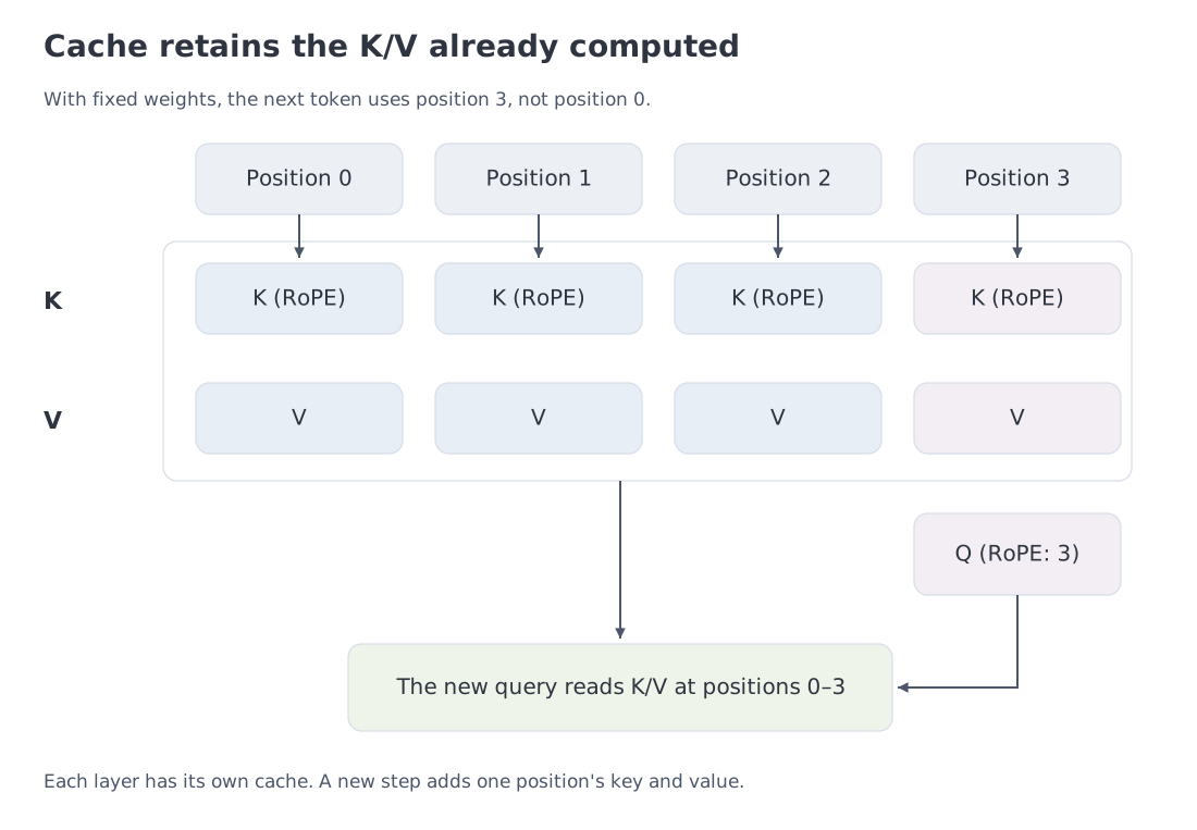
Figure 5. Caching changes execution order and storage. It does not add a learned memory parameter to the network.

15. MoE replaces a specific operator

Module 7 introduced experts as a replacement for the dense FFN. We can now identify the exact substitution: replace $\mathcal F_\ell$ in Section 7 by $\mathcal F_{\rm MoE,\ell}$. With all other settings held fixed, attention, residual connections, the vocabulary head, and the autoregressive factorization remain unchanged.

Consider MiniLLM's sigmoid router without an expert-capacity limit. With $E_r$ routed experts, the router matrix has shape $W^r\in\mathbb R^{d\times E_r}$. For a normalized row $y$, let $r=yW^r$ and $a_e=\sigma(r_e)$. A balancing offset $b_e$ affects the selected set $S(y)=\operatorname{TopK}_e(a_e+b_e)$, while mixture weights use the original sigmoid scores:

$w_e(y)=\frac{a_e}{\varepsilon_r+\sum_{j\in S(y)}a_j},\quad e\in S(y),\qquad\mathcal F_{\rm MoE}(y)=\sum_{e\in S(y)}w_e(y)\mathcal F_e(y)+\sum_{e\in\mathcal S_{\rm shared}}\mathcal F_e(y).$

MiniLLM uses the denominator stabilizer $\varepsilon_r=10^{-9}$. Without it, selected weights would sum exactly to one; with it, their sum is slightly smaller. For ordinary scores this is a small numerical correction, but it matters when all selected sigmoid scores are nearly zero. Each expert is a separate SwiGLU. Shared experts in $\mathcal S_{\rm shared}$ always run and are summed without normalization in this configuration. Other implementations may scale those contributions differently; that scaling belongs in their equations.

Take router logits $(0,1,-1)$, offsets $(0,-0.5,0.5)$, and top-2 selection. Sigmoid scores are $(0.5,0.731059,0.268941)$, whereas selection scores are $(0.5,0.231059,0.768941)$. Experts 2 and 0 are chosen. Their normalized weights are approximately $(0.349755,0.650245)$. Including the balancing offsets in this normalization would define a different router.

Within a region where the selected set stays fixed, gradients pass through the selected expert outputs and their mixture weights. Top-k itself is discrete; ordinary smooth derivatives do not describe a change of selected set at a boundary. MiniLLM updates balancing offsets through a separate control rule, rather than through AdamW on cross-entropy. They are routing state, distinct from the gradient-trained matrices in $\theta$. We have excluded capacity limits and token dropping because they add dependencies on the assignments and ordering within a batch.

16. Other objectives and the boundary of the model

SFT can leave the entire forward pass intact while selecting only response targets through $b_t$. Prompt tokens remain visible to attention: excluding a target from the loss does not remove its token from the context. LoRA changes the parameterization of selected matrices. For $W_0\in\mathbb R^{d_{\rm in}\times d_{\rm out}}$, write $W=W_0+(\alpha/r)AB$, with $A\in\mathbb R^{d_{\rm in}\times r}$, $B\in\mathbb R^{r\times d_{\rm out}}$, adapter rank $r\gt0$, and specified scale $\alpha$. The frozen $W_0$ participates in computation while the optimizer updates the adapter matrices.

Preference learning can change the objective itself. For DPO, define $\ell_\theta(y\mid c)=\sum_i\log p_\theta(y_i\mid c,y_{\lt i})$, the sum of response-token log probabilities conditioned on prompt $c$. Let $y^+$ be preferred to $y^-$ and let $\pi_{\rm ref}$ be a fixed reference model. Write $\ell_{\rm ref}$ for the corresponding response log-probability sum under that model. The loss for one pair is

$\mathcal L_{\rm DPO}=-\log\sigma\!\left(\beta\left[\ell_\theta(y^+\mid c)-\ell_\theta(y^-\mid c)-\ell_{\rm ref}(y^+\mid c)+\ell_{\rm ref}(y^-\mid c)\right]\right).$

Here $\beta\gt0$ sets the scale of the comparison. Replacing response log-probability sums by length-normalized averages would change this objective. Module 14 develops the derivation and limitations. For the synthesis, the key point is that the same forward distribution can support different learning objectives.

A multimodal model may insert image or audio projections into its input sequence instead of using only rows of $E$. Retrieval supplies documents to the context. An agent controller calls tools and constructs a subsequent request. None of these behaviors is supplied automatically by the final multiplication by $U$. The core equation describes a probability computation; it does not certify factual accuracy, retrieval quality, or system reliability. That is why the course also needs the evaluation methods of Module 19.

19. Where the construction changes: SSMs and diffusion

An SSM carries a different representation of the past

Attention retains separate key/value records for past positions and reads them according to the current query. A state space model, or SSM, carries a state whose shape is fixed by the architecture. A discrete state-space core can be written as

$s_p=\overline A_p s_{p-1}+\overline B_p u_p,\qquad y_p=C_p s_p+D u_p.$

For this local recurrence, use column vectors: input $u_p\in\mathbb R^{d_u}$, state $s_p\in\mathbb R^n$, and output $y_p\in\mathbb R^{d_y}$. The coefficient shapes are $\overline A_p\in\mathbb R^{n\times n}$, $\overline B_p\in\mathbb R^{n\times d_u}$, $C_p\in\mathbb R^{d_y\times n}$, and $D\in\mathbb R^{d_y\times d_u}$. Selective models make some coefficients depend on the current input. The bars indicate coefficients already expressed in discrete time; Module 8 explains the connection to continuous dynamics.

For a transparent scalar case, choose $\overline A=0.5$, $\overline B=C=1$, $D=0$, and $s_{-1}=0$. Inputs $(1,0,-1)$ produce states and outputs $(1,0.5,-0.75)$. Earlier inputs affect the result through the state, rather than through individually addressable K/V records. State size need not grow with prefix length; that does not mean it preserves every detail of an arbitrarily long history without loss.

The stack must now contain an SSM block wherever that context-processing mechanism is used. A full Mamba block is not obtained merely by replacing the product $QK^\top$: it can include projections, convolution, and gating, and need not have a separate FFN. A hybrid can interleave different block types. Yet if the model still predicts the next token causally, the vocabulary softmax, autoregressive product, and token cross-entropy retain their meaning. The principal changes are the context operator and the state carried between positions. Mamba provides a concrete architecture built around this idea.

Diffusion changes the route from randomness to a sequence

Diffusion changes more than the way a prefix is represented. Let $z^{(s)}$ denote an entire sequence at noise level $s$, so this index cannot be confused with a token position. The clean sequence is $z^{(0)}$. Start with $z^{(S)}$ drawn from a specified noise distribution; a masking process may start with all MASK tokens. A denoiser receives the current sequence and its noise-level information, rather than only an immutable left prefix.

Let $K_{\theta,s}(z^{(s-1)}\mid z^{(s)},c)$ be the normalized reverse transition conditioned on prompt $c$. For a fixed sequence length,

$\boxed{p_\theta(z^{(0)}\mid c)=\sum_{z^{(1)},\ldots,z^{(S)}}p_S(z^{(S)}\mid c)\prod_{s=1}^{S}K_{\theta,s}(z^{(s-1)}\mid z^{(s)},c).}$

The product describes a single refinement trajectory. The sum accounts for all hidden intermediate sequences that could lead to the same clean result. Continuous-noise versions use corresponding integrals. If length is also generated, its distribution must be modeled separately.

A denoiser often predicts clean-token probabilities, while the transition $K$ additionally depends on the corruption process and schedule. We therefore cannot automatically identify $K$ with a single token softmax. Attention may also become bidirectional: positions can read the available noisy state across the sequence. Simply removing a causal mask while asking a network to copy visible correct tokens would leak targets rather than define a valid diffusion task. In Module 12, training reconstructs hidden tokens from corrupted inputs; more generally, the objective follows the chosen forward corruption process and reverse-model formulation. D3PM develops this discrete setting.

To make marginalization tangible, consider a hand-specified reverse chain, not a trained denoiser. Two binary positions have four possible strings: 00, 01, 10, 11. From two MASK symbols, the first transition produces $r=(0.18,0.42,0.12,0.28)$. The second transition independently keeps each bit with probability 0.8 and flips it with probability 0.2. For strings differing in $h$ positions, the transition probability is $0.8^{2-h}0.2^h$. Multiplying $rK$ gives $(0.2128,0.3472,0.1672,0.2728)$. For instance, the probability of 00 is $0.18\cdot0.64+0.42\cdot0.16+0.12\cdot0.16+0.28\cdot0.04=0.2128$. This adds four possible paths; it is not a prediction of the first bit followed by a prediction of the second.

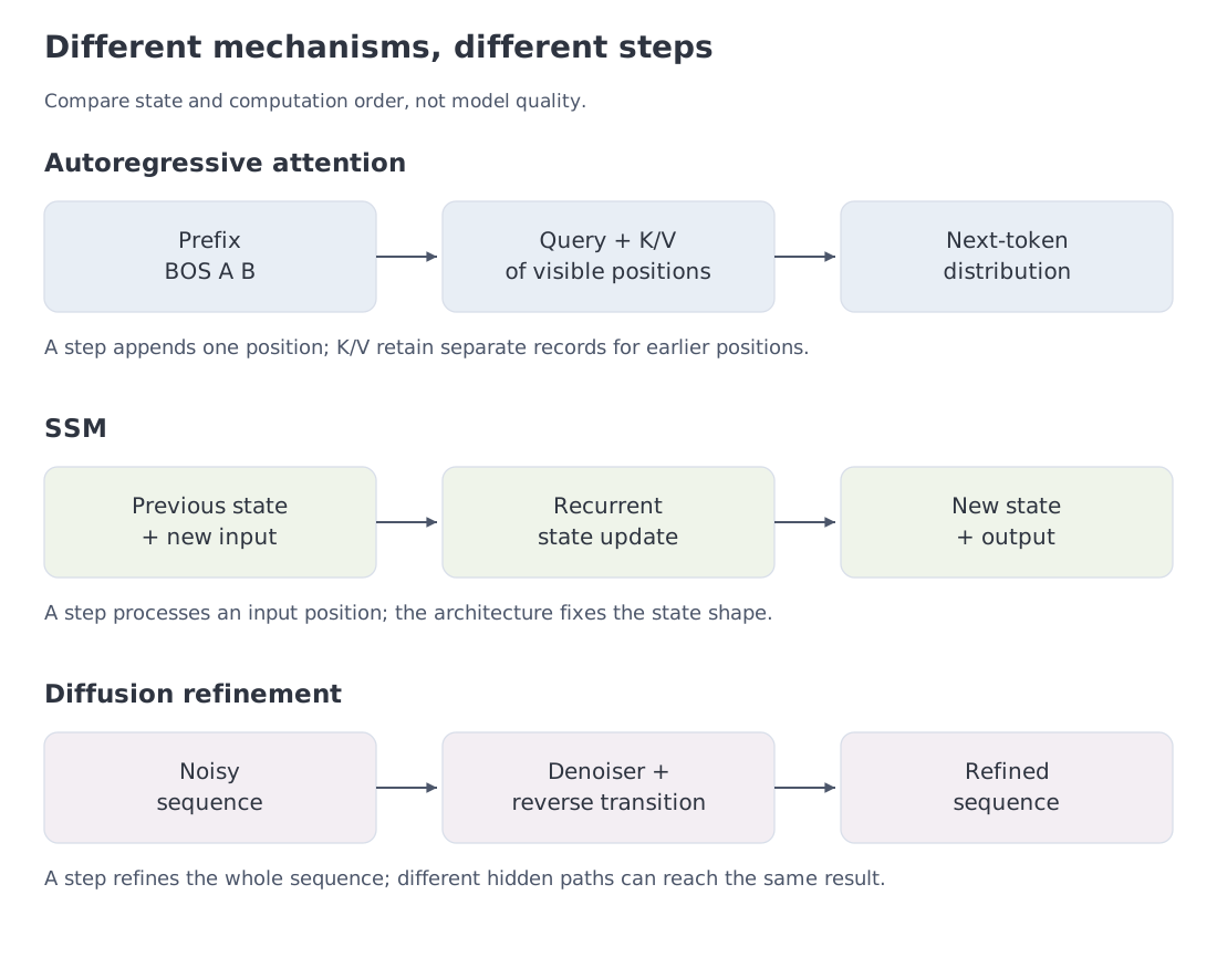
Figure 6. An SSM can retain an autoregressive objective. A diffusion refinement step concerns a complete sequence, whose changing representations generally prevent reuse of an ordinary append-only KV-cache.

Any normalized joint distribution admits a chain-rule factorization into token conditionals. That identity does not make a diffusion sampler autoregressive: evaluating those conditionals may require marginalizing hidden trajectories. Denoiser architecture, probabilistic model, and sampling algorithm are related descriptions, but they are not interchangeable.

20. The final expression, with its meaning intact

Return to the dense MiniLLM configuration. Write $\mathcal T_G(H)=H+G(H)$ for residual addition. A block is then $\mathcal B_\ell=\mathcal T_{\mathcal F_\ell\circ N_{\gamma_{f,\ell}}}\circ\mathcal T_{\mathcal A_\ell\circ N_{\gamma_{a,\ell}}}$. Sections 5–7 have already expanded every operation inside $\mathcal A$ and $\mathcal F$. The conditional distribution is

$\boxed{p_\theta(x_t=v\mid x_{\lt t})=\left[\operatorname{softmax}\!\left(\left[N_{\gamma_o}\!\left((\mathcal B_L\circ\cdots\circ\mathcal B_1)(E[x_{\lt t}])\right)\right]_{t-1,:}U\right)\right]_v.}$

Read it from the inside outward: look up prefix embeddings; apply the fully defined blocks in order; normalize; select the last row; project to vocabulary logits; normalize those logits; take the component for token $v$. A training pass keeps all rows for its target predictions rather than selecting only the last one.

Multiply the conditionals to obtain a sequence probability. Choose a loss and differentiate it to train. Transform the final distribution into $q$ and select a token to generate. The complete procedure is expressed by the following connected equations:

$\boxed{\begin{aligned}p_\theta(x_{1:N}\mid x_0)&=\prod_{t=1}^{N}p_\theta(x_t\mid x_{\lt t}),\\\mathcal L(\theta)&=-\frac{1}{\sum_t b_t}\sum_t b_t\log p_\theta(x_t\mid x_{\lt t}),\\(\theta_s,m_s,v_s)&=\operatorname{AdamW}_s\!\left(\theta_{s-1},m_{s-1},v_{s-1},\nabla_\theta\mathcal L(\theta_{s-1})\right),\\x_t&\sim q_\theta(\,\cdot\mid x_{\lt t})\quad\text{with weights held fixed.}\end{aligned}}$

The AdamW operator here includes the clipping rule, learning-rate schedule, and decay groups defined in Section 12. The last line describes sampling; greedy decoding substitutes argmax. These lines are not executed simultaneously: training produces new weights, while generation uses a chosen checkpoint.

The expression now has a precise scope. MoE replaces $\mathcal F$ and adds routing. An SSM changes a block and its carried state while retaining the autoregressive objective when that objective is chosen. Diffusion uses a different generation trajectory and a distribution over hidden refinement states. Architecture specifies a computation; scale, data, and optimization determine what its parameters learn. The equation does not predict a model's capability level on its own, but it does let us locate every operation, learned quantity, and surrounding algorithm.

Sources and the next practical step

Modules 3–9 and 12–14 contain the detailed treatments of individual mechanisms. Primary descriptions include Attention Is All You Need, RMSNorm, RoFormer, GQA, AdamW, and DPO. This module specifies a particular educational MiniLLM configuration; its numerical matrices were created for the running example.

Finish with the self-check questions. The first route includes the 13 unlabelled questions; return to 20.11.1 after the detailed backward pass in Section 11 and to 20.15.1 after the router in Section 15. Then revisit the MiniLLM capstone and map its config.json to the equation. A change in head count, embedding tying, or FFN type should now correspond to an explicit change in dimensions, operations, and parameters that you can verify computationally.