Module 9. Pretraining: Data, Scaling Laws, and Optimizers
“Modern LLMs” course · Module 9 lecture · edition 2026.10.25
What this module is about. The previous modules assembled the machine: tokenization, positional mechanisms, attention, Transformer blocks, mixture-of-experts routing, and alternative architectural branches. A model with those components is still only an untrained dynamical system. Pretraining is the stage at which architecture, data, optimization, numerical precision, and cluster topology must work together for months without a cheap reset button.
We will follow three decisions that belong to the same training run. What data should the model see? How should a fixed compute budget be divided between parameters and tokens? Which optimization and systems choices can carry the run through trillions of tokens without instability? The mathematical path starts from , derives the analytic optimum of a particular Chinchilla-style fit, measures the cost of moving away from that optimum, and adds inference to the lifecycle objective. The practical path covers data curation, Muon, MuonClip, µP-style transfer, and the memory accounting behind ZeRO/FSDP. We use these mechanisms to read large-run reports and their resource constraints. Implementing a distributed training runtime or GPU kernels requires a separate course.
The module distinguishes exact algebra inside an assumed model from empirical fit, vendor-reported run results, and broader conclusions. That distinction matters more at frontier scale, where a memorable number can travel farther than the conditions under which it was measured.
Useful background. Modules 3 and 6 explain the computation and decoder block; Modules 5 and 7 provide the attention and expert-parallel context. For the compute estimates here, distinguish work in FLOP from throughput in FLOP/s: their ratio gives compute time. Device utilization, communication, and data movement reduce sustained throughput below the hardware peak. Module 10 develops the fuller roofline model.
Reading routes
- First pass: read §§1–3 and 5 for the problem and the data pipeline. In §4, focus on the variables and final allocation formula; continue with §§6–11 and 15, then try Q1–Q7 in §18 and E1–E3. Return to Q8 after reading the run passports in §17.
- Second pass: work through the derivation in §4 and execute the code and notebooks in §§12–13. Follow with hyperparameter transfer (§14), precision (§16), and selected run reports (§17).
- Reference: use §4 for equations, §§10–11 for optimizer mechanics, §15 for state accounting, and §20 for sources. The run reports can be read independently.
Pretraining builds a base model from a large data mixture, usually through next-token prediction. Later training that shapes its behavior is a separate stage.
1. Motivation: three irreversible choices
Imagine that the model code has passed small-scale tests and a large cluster has been reserved for several months. “Train the model” now decomposes into a sequence of choices whose mistakes are expensive in different ways.
The first choice is the training distribution. The web does not arrive as a textbook. It contains duplicated pages, navigation fragments, generated spam, broken encodings, private information, and documents that are grammatical yet nearly useless as learning signal. A corpus is therefore not something found; it is something manufactured through extraction, filtering, deduplication, scoring, policy checks, and mixture design.
The second choice is the allocation of compute. With a fixed FLOP budget, one can train a larger model for fewer tokens or a smaller model for longer. Neither extreme is automatically attractive. Too few parameters impose a capacity penalty; too few tokens leave capacity underused. Scaling laws turn this trade-off into an empirical optimization problem, but the objective must be stated carefully. Chinchilla asks for the lowest fitted loss at a fixed training budget. A product team may care instead about total lifecycle cost after the model has generated trillions of tokens.
The third choice is the update rule and its numerical environment. A brief instability in a toy experiment costs minutes. A divergence after ten trillion tokens can cost days of cluster time, checkpoint recovery, and forensic debugging. Optimizer geometry, learning-rate schedule, precision policy, and monitoring therefore form one control system rather than four independent implementation details.
The choices interact. Data quality changes the observed scaling curve. The chosen parameter/token ratio changes future serving cost. The optimizer determines whether the planned token horizon is reachable. A strong pretraining recipe is not a bag of individually good techniques; it is a coherent design whose assumptions agree.
2. The historical arc: the objective kept expanding
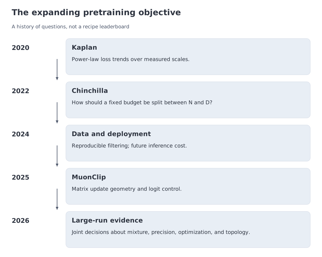 From Kaplan’s empirical power laws to Chinchilla’s compute-optimal balance, inference-aware allocation, reproducible data pipelines, Muon/MuonClip, low-precision pretraining, and the 2026 public run reports.
The modern story begins with a narrower question than the one posed in this module. Kaplan et al. showed in 2020 that language-model loss followed smooth power-law trends over the model, data, and compute ranges they studied. Their fitted regime encouraged parameter growth faster than token growth and matched the design instincts of the GPT-3 era: very large models trained on corpora that now look comparatively small.
Chinchilla revisited the allocation in 2022 with a broader experimental sweep. Its central practical message was that many large models were undertrained on data. Under a fixed training-compute budget, parameter count and token count should grow in a much more balanced way. “About twenty tokens per parameter” became a convenient mnemonic for the studied range, although neither the paper nor the mathematics made it a timeless constant.
The next expansion added deployment. A model is trained once but may be invoked billions of times. If two configurations reach comparable quality, a smaller model trained for longer can spend more compute up front and repay it through cheaper inference. This lifecycle view explains why a run such as Llama 3 8B on more than 15T tokens can be economically sensible even when it lies far to the data-heavy side of a historical compute-optimal fit.
At the same time, the symbol stopped looking like an interchangeable pile of tokens. FineWeb, FineWeb-Edu, DCLM, Nemotron-CC, and later multilingual corpora such as FineWeb2 made data construction itself a reproducible research object. The question shifted from “how much web text?” to “which documents, with which filters, mixture weights, provenance, and evaluation loop?”
Optimization became more visible as runs grew longer. AdamW remained a strong default, but matrix-aware methods such as Muon appeared in public frontier-scale training stacks. Kimi K2 documented MuonClip and a 15.5T-token run without loss spikes. DeepSeek V4 reported Muon alongside mHC and hybrid attention. Kimi K3 extended the line with head-wise treatment inside the optimizer. These examples do not establish a universal winner; they establish that matrix-geometric optimization became operational at trillion-parameter scale.
Infrastructure evolved in parallel. ZeRO and FSDP reduced replicated state, multi-axis parallelism became normal, FP8 appeared in public large-scale pretraining, and NVIDIA documented NVFP4 pretraining in Nemotron 3. The historical pattern is therefore not a sequence of single-algorithm replacements. The objective expanded: predict loss, allocate compute, account for inference, curate data, preserve numerical stability, and map the whole state onto a cluster.
3. Three classical ideas hiding inside frontier pretraining
The scale is new; much of the logic is not.
An empirical law is a model of a regime
A relation such as
has an exact straight-line form after subtracting the floor: for and , . Plotting itself is only approximately linear where dominates . Fitting such a relation can compress many experiments into a few coefficients. That is the appeal of scaling laws. It is also the danger. A fit is only as universal as the architectures, tokenizers, datasets, numerical formats, and scale range behind it. Kaplan and Chinchilla are a useful reminder that a smooth line may change when the experimental regime changes.
A responsible use of a scaling law therefore has three layers: fit the observed region, optimize the fitted function, and label any extrapolation beyond the observed region. The second step can be exact mathematics while the third remains uncertain science.
Corpus construction is sampling theory at industrial scale
Classical ML already taught us to inspect duplicates, outliers, missing values, class imbalance, and train/test contamination. Web-scale pretraining encounters the same categories with documents rather than rows and billions rather than thousands of examples.
The scale changes the algorithms. Pairwise document comparison is impossible, so near-duplicate search uses shingles, MinHash signatures, and locality-sensitive hashing. Human quality labels cannot cover the corpus, so a small labeled set trains a cheaper classifier that scores the rest. Domain weights resemble stratified or importance sampling, except that the objective is a general-purpose foundation model rather than one fixed target label.
Optimizers exploit different geometries
It is useful to separate three families rather than place every method on one “approximate Hessian” ladder.
- First-order methods with gradient history, such as AdamW and Lion, adapt updates in different ways: AdamW rescales by moment estimates, while Lion uses the sign of a momentum-based update.
- Preconditioning or curvature-oriented methods, such as Shampoo, SOAP, and Sophia, construct richer approximations to local geometry.
- Matrix-geometric methods, represented here by Muon, transform a momentum update using the fact that many parameters are matrices.
Muon does not explicitly build a Hessian. Its practical operation is easier to understand through singular values: it turns a highly anisotropic matrix update into one with a much narrower spectrum. That is the mechanism we will derive in §10.
Optional depth. Cross-entropy, KL divergence, coding length, and the limits of interpreting loss as “information learned” are developed in Information Theory for ML. The present module remains self-contained and uses cross-entropy only as the measured pretraining objective.
The calculations use mean cross-entropy in nats per token. Enter and as counts, not as numbers measured in billions. Table suffixes B and T mean and . Loss values from different tokenizers are not directly comparable.
4. Formalism: compute, a fitted loss surface, and its analytic optimum
We begin with a dense-model approximation. Let
- be the parameter count;
- the number of training tokens;
- the total floating-point operation count.
A common first-order estimate is
The intuition is roughly operations per token for the forward pass and another for the backward pass. This is not an accounting identity for every architecture. Long-context attention, sparse experts, embeddings, checkpointing, recomputation, and optimizer work add model- and system-specific terms. The approximation is useful because it exposes the dominant parameter–token trade-off.
Take the following rounded Chinchilla-style fit:
with
The terms have a simple interpretation. is the fitted irreducible floor. is the capacity penalty. is the data penalty.
At fixed , eliminate :
The loss along the iso-compute curve is
The first penalty falls with . The second rises because a larger model leaves fewer tokens under the fixed budget. Differentiating gives
Set the derivative to zero:
Hence
The star denotes the exact optimum of this rounded fitted function under the assumption . The algebra is exact inside the model; the model itself is empirical.
The scaling exponents follow immediately:
Because in this parameterization, the optimal token count grows slightly faster than the optimal parameter count, and
drifts upward with the budget. The familiar twenty-token ratio is therefore not a mathematical invariant of this fit.
5. From raw web pages to a training distribution
Calling a corpus a “dataset” can make it sound like a static file. In practice it is the output of a long decision pipeline. Follow one hypothetical page through that pipeline.
5.1 Extract the document and identify its language
The useful text must be separated from menus, consent banners, advertisements, repeated navigation, and footer material. A language identifier then estimates which language or languages the document contains. A single global threshold is rarely adequate for a multilingual corpus because classifier quality, script, and typical document length differ by language. FineWeb2 illustrates why per-language calibration matters when the goal extends far beyond English.
5.2 Remove obvious structural junk
Heuristics catch documents that parse successfully but do not resemble useful prose or code: repeated character runs, keyword lists, malformed markup, anomalous word lengths, excessive n-gram repetition, or pages dominated by boilerplate. Gopher-style pipelines use many such rules.
The thresholds are engineering choices, not universal constants. A repetition rule that works for web prose may destroy source code or tabular data. Mature pipelines therefore evaluate filters through small-model training and downstream metrics rather than visual cleanliness alone.
5.3 Deduplicate across documents
A shingle is a short sequence of adjacent words or tokens. For shingle sets and , Jaccard similarity is . MinHash compresses the sets while approximately preserving this similarity; locality-sensitive hashing (LSH) finds likely matches without an exhaustive pairwise scan. Candidate detection still needs a retention policy.
Licenses, syndicated news, mirrored documentation, e-commerce templates, and copied articles can appear across thousands of domains. Repetition wastes training mass and increases the chance of benchmark contamination.
All-pairs comparison is infeasible. Documents are represented by shingle sets, compressed into MinHash signatures, and grouped through locality-sensitive hashing. Candidate near-duplicates can then be compared more carefully, and each cluster can retain the most complete or highest-quality representative.
5.4 Estimate learning value with a model
Heuristics recognize junk better than they recognize educational value. A common pattern is to label a manageable sample with humans or a stronger model, train a cheaper classifier, and apply it at scale.
FineWeb-Edu is a clear example. Llama 3 70B scored the educational value of roughly 460,000 documents; those labels trained a scalable classifier used on the larger pool. The resulting educational slice contains about 1.3T tokens, compared with roughly 15T in full FineWeb. The LLM acts as a costly teacher for a cheaper filter rather than as the corpus generator.
5.5 Apply safety, privacy, and legal policy
Quality and admissibility are different axes. Email addresses, phone numbers, identifiers, and other personally identifiable information (PII) may be detected with regular expressions and named entity recognition (NER) systems. Toxicity or policy categories require classifiers and an explicit governance decision. A high-quality document may be excluded for policy reasons; a harmless document may still be useless for training.
5.6 Build the mixture and its schedule
A clean document collection still does not define the distribution seen by the model. The team must choose the relative weight of code, mathematics, science, conversational text, books, and languages. The mixture may change over the run: broad coverage early, then higher-quality or domain-targeted data during a late annealing phase.
Several public artifacts should not be compared as though they were the same object:
- FineWeb contains about 15T tokens of filtered English web text; FineWeb-Edu is a roughly 1.3T-token educational subset.
- FineWeb2 extends the approach to more than a thousand languages and reports roughly 20 TB of text / about five billion documents; token count depends on the tokenizer.
- Nemotron-CC is published as a family totaling about 6.3T tokens and includes quality classification plus synthetic rewriting of part of the corpus.
- DCLM is a benchmark and standardized candidate pool of roughly 240T tokens for comparing data-selection strategies. DCLM-Baseline used 2.6T training tokens. The candidate pool and the token count of one training run are different passport fields.
Code, mathematics, scientific documents, and multimodal data usually require specialized branches: parser-aware extraction, license checks, execution or formal verification, perceptual deduplication, and image–text alignment.
The preprocessing system is also a software supply chain. Dataset loaders and conversion tools execute code and may access external storage. A July 2026 Hugging Face incident demonstrated that a data-processing path could become an intrusion path. Immutable images, allow-listed loaders, restricted network egress, secret isolation, pinned versions, and configuration review therefore belong to corpus engineering as surely as quality filters do.
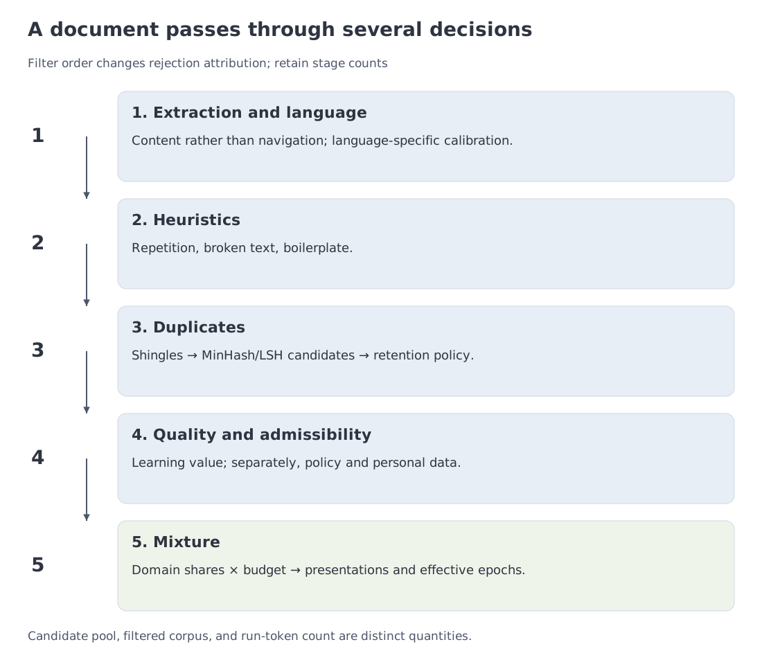 Extraction and language identification → heuristics → near-duplicate removal → model-based quality scoring → privacy/policy checks → domain mixture. The diagram distinguishes a candidate pool from the token count of a particular training run.
6. Worked example A: two budgets and the cost of a mnemonic
The analytic expression in §4 and the popular rule answer similar-looking questions in different ways. Let us compare them explicitly.
If we impose and combine it with , then
The arithmetic is internally consistent, but the token-to-parameter ratio was fixed before optimization. The fitted loss surface does not impose that ratio; it produces one from its coefficients and the selected budget.
| Training budget | Analytic | Analytic | Imposed : , | |
|---|---|---|---|---|
| FLOP | 35.7B | 3.38T | 94.7 | 77.6B, 1.55T |
| FLOP | 63.6B | 6.82T | 107.2 | 147.2B, 2.94T |
The first budget is the rounded value of the 8.03B/15T teaching scenario. The second is a separate illustrative FLOP budget; it is not a hardware runtime estimate.
The gap is not evidence for a new “correct” ratio of one hundred tokens per parameter. It is evidence that three objects must not be conflated:
- a convenient rule of thumb;
- the optimum of one rounded 2022 fit;
- the design point selected for a new architecture and a new data mixture.
A real team builds its own iso-compute curves with proxy models and its own corpus. The closed-form calculator remains valuable because it makes the reasoning transparent and catches arithmetic errors. It is not a substitute for those experiments.
7. The isoFLOP valley and the fitted cost of long training
At fixed , every parameter count determines exactly one token count, . We can therefore plot the fitted loss along a one-dimensional isoFLOP curve.
On the left, the model is small and the capacity term dominates. On the right, the model is large but receives too little data, so the data term dominates. Between them lies a broad valley.
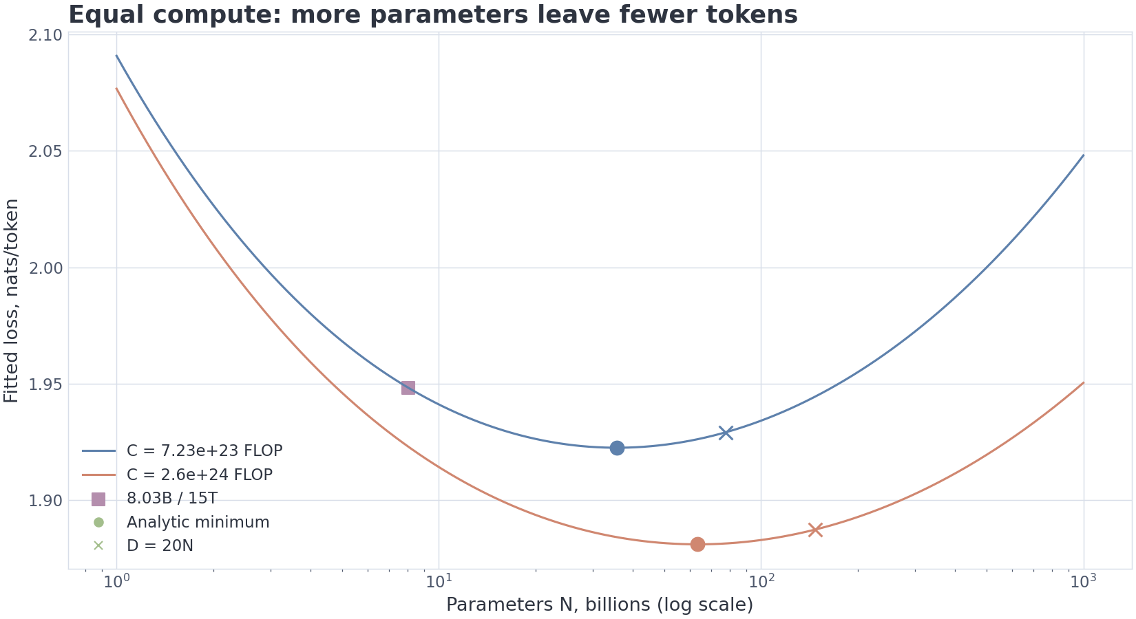 IsoFLOP curves for two budgets. The analytic optimum, the imposed 20-token rule, and the 8.03B/15T point are shown on the same fitted surface.
The shape of the valley matters for lifecycle design. Moving toward a smaller model and more tokens can add relatively little fitted loss while reducing the active parameter count—and therefore the cost of every future dense decode token.
Take
Under the dense approximation,
This is about 1,868 training tokens per parameter. The analytic optimum of the same fit at the same budget is
The fitted losses are
and
Taking the difference before rounding the losses gives
This number is a counterfactual inside the selected fit. It is not a measured penalty of Llama 3 8B and does not claim that the real team “paid 0.0258 loss.” The architecture, data mixture, and training recipe differ from the experiments behind the coefficients. The calculation says only: if we take this fitted surface literally, moving from 35.7B/3.38T to 8.03B/15T raises fitted loss by 0.0258 while making the model about 4.4 times smaller.
That exchange cannot be judged from training alone. The smaller model keeps saving compute after release; the next section asks when those savings repay the additional pretraining.
8. Inference-aware allocation: when does the smaller model repay its training?
Change the comparison. Instead of asking for the lowest fitted loss at a fixed training budget, ask for two models that reach the same fitted target.
Use the 8.03B/15T value
A 70B model reaches the same fitted value after solving
The result is
Its training cost is
Inside this model, the 70B configuration reaches the target with about 36% less training compute than the 8.03B/15T configuration. If the model were trained once and never served, the larger model would win this comparison.
Now add dense decoding. Approximate one generated token by FLOP. The smaller model spent an extra
during training. The larger model spends an extra
on every generated token. The break-even volume is
Beyond roughly 2.12T generated tokens, the 8.03B configuration becomes cheaper in the sum of training compute plus this simple dense-decode estimate.
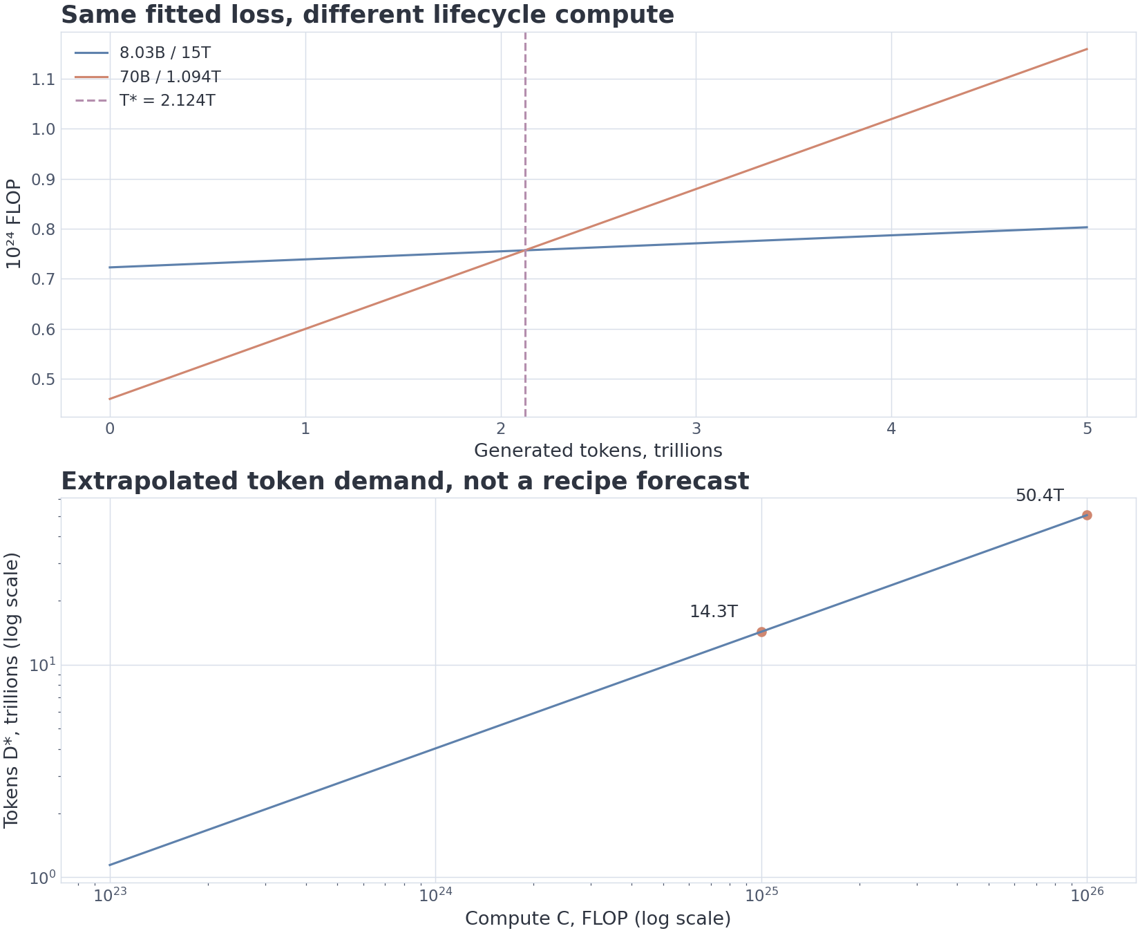 Lifecycle compute for two equal-fitted-loss configurations, and the token demand implied by extrapolating the selected fit to larger budgets.
The simplification omits batching, memory bandwidth, KV cache, quantization, speculative decoding, and the possibility that equal average loss does not mean equal task utility. The point is methodological: the training-compute optimum and the product-cost optimum need not coincide.
Inference-aware scaling does not refute Chinchilla. It changes the objective from “minimize fitted loss under a training budget” to “minimize lifecycle cost under a quality target and an expected usage volume.”
9. The data wall: token counts stop being interchangeable
Extrapolating the fitted optimum produces about 14.3T tokens at and about 50.4T at . These are not forecasts of a frontier recipe. They illustrate a structural tension: compute can grow faster than the supply of high-quality, sufficiently independent, legally usable data.
A raw token, a filtered token, and a token that provides genuinely new learning signal are not the same quantity. Ten copies of the same article increase the literal counter by ten but contribute far less than ten independent observations. A superficial rewrite changes the surface form without necessarily changing the underlying information.
Several responses address different parts of the problem.
Optimize the mixture rather than treating it as fixed
DoReMi treats domain weights as tunable variables. A proxy model estimates which domains suffer the largest excess loss relative to a reference, and the mixture is adjusted accordingly. The method does not discover an objective universal mixture: its result depends on the domain partition, proxy model, and evaluation target. It does turn part of curation into a reproducible optimization loop.
Reuse the best data, but track diminishing returns
Repeated epochs can still help when data is scarce, especially on high-quality subsets. The marginal value falls, however, because later exposures resemble earlier ones. It is therefore useful to distinguish literal token presentations from effective new data.
Many recipes combine repetition with scheduling: broad coverage first, then a late high-quality or domain-specific phase. This is closer to curriculum design than to blindly replaying the whole corpus.
Transform documents into denser training signal
Synthetic data can turn a weak page into a structured explanation, a verified code problem, a dialogue, or a cleaned rewrite. The benefit depends on verification and diversity. Model-generated text can also amplify the teacher’s mistakes, style, and blind spots; “synthetic” is not a synonym for “high quality.”
For code and mathematics, executable or formally checkable outputs are especially valuable. They attach a verification channel to the generated example rather than relying only on linguistic plausibility.
Add reasoning trajectories carefully
Reasoning traces may provide intermediate supervision and expose how a solution unfolds. They can also be long, persuasive, and wrong. The useful unit is not “a chain of thought” in the abstract but a trajectory whose outcome or intermediate steps can be checked.
Connection to RL. This section treats reasoning trajectories as data. Their generation through RLVR/GRPO, verifiable rewards, and large rollout systems is developed in RL for LLM, Modules 9–10. The information-theoretic view of reasoning signal is developed in Information Theory for ML, Module 13.
A note on diffusion language models
A masked diffusion language model can revisit the same document under different masks and therefore solve a different conditional reconstruction problem on each exposure. That can create more varied supervision than replaying the same left-to-right factorization. It does not guarantee superiority in every data-limited regime; usefulness depends on the objective, architecture, and whether the new masks impose informative constraints.
The “data wall” is not a date on which the internet runs out. It is a gradual decline in the marginal value of the next token and a rise in the cost of cleaning, licensing, verifying, and scheduling it.
The notebook makes repetition concrete. A 15T-token run with a 15% mathematics share allocates 2.25T token presentations to mathematics. A unique pool of 0.4T tokens therefore receives effective epochs. This measures average reuse, not the arrival of 5.625 new corpora.
10. Muon: change the spectrum of a matrix update
AdamW remains a strong and well-understood baseline. Its practical advantage is coordinate-wise adaptation: parameters with different gradient histories receive different effective step sizes.
The learning rate controls the overall step size. Momentum carries a decaying history of gradients, smoothing changes in direction. Weight decay shrinks the parameters themselves. AdamW applies that shrinkage separately from its adaptive gradient scaling, so adding an L2 penalty to the loss generally produces a different update.
Second pass: trace one AdamW step
Write for the parameters and for the loss gradient. Initialize two running averages at , with decay coefficients . All operations are coordinate-wise:
The hats correct for initializing the averages at zero. Here controls weight decay and keeps the denominator positive. This is the common API convention in which decay is multiplied by the current learning rate.
For , , , , , , and , the first result is approximately . Decay alone gives ; the adaptive term contributes roughly . The notebook follows another step after the gradient changes sign, exposing the role of history. AdamW.
Large Transformer parameters, however, are naturally matrices. Attention and MLP projections are not merely long vectors with arbitrary reshaping. Suppose a matrix update has a few dominant singular directions and many weak ones. A step can then concentrate most of its effect in a narrow subspace.
Muon begins with a momentum-like update
For a two-dimensional parameter, it then approximates a polar factor
Here is the update matrix and SVD means singular value decomposition. The inverse-square-root expression requires full row rank; a tall matrix has singular . In general, use the pseudoinverse square root and retain zeros in null directions. The expression uses the compact SVD on the nonzero singular subspace. The code transposes tall inputs so the Gram matrix is only .
If , the ideal polar factor is . The singular-vector directions remain; the nonzero singular values are replaced by ones. In practical terms, Muon narrows the spread of singular values and makes the update more isotropic in matrix geometry.
The momentum equation isolates accumulation. A complete implementation also chooses momentum normalization, optional Nesterov mixing, shape-dependent step scaling, and weight decay. The notebook starts with a prepared update matrix. GEMM means matrix multiplication; the five iterations below are only one part of an optimizer step.
Computing an SVD for every large matrix on every step would be too expensive. Muon therefore uses a small number of Newton–Schulz matrix iterations implemented through GEMM. The teaching trace uses the quintic coefficients
and the normalized recurrence
For the fixed matrix in the notebook, the initial singular-value spread is about 5.1 (). After five quintic iterations, the spectrum lies roughly in .
This is not an exact orthogonal factor. remains nonzero. Three additional classical cubic iterations can move the band to approximately , but exactness costs more GEMM work. An optimizer needs a useful geometric transformation, not a perfect numerical linear-algebra result.
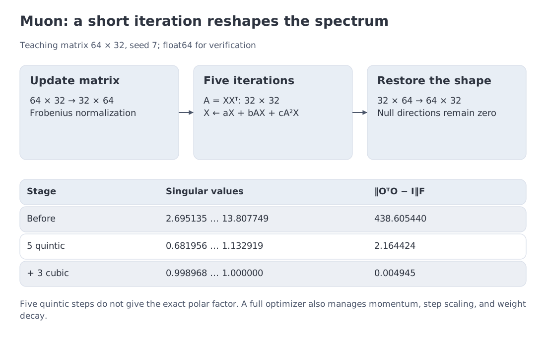 Momentum update → five Newton–Schulz quintic iterations → a much narrower singular-value band. The inset contrasts the practical approximation with near-exact orthogonalization.
Calling Muon “second order” can obscure more than it clarifies. Some analyses connect it to Newton-like geometry, but the practical algorithm does not construct a Hessian. The robust statement is narrower: Muon exploits the matrix structure of the update and changes its spectrum.
Public large-scale recipes are usually hybrid. Large matrices may use Muon, while embeddings, normalization parameters, biases, and other tensors remain on Adam or AdamW. “The model optimizer” can therefore mean a parameter-class policy rather than one update rule applied everywhere.
11. MuonClip: correct the parameter source of unstable attention logits
Spectral normalization of the update does not prevent every instability. During Kimi K2 scaling, the developers observed attention heads whose query–key logits grew over time. Large-magnitude values drive softmax toward saturation and can turn a local head-level problem into a loss spike.
Clipping the logits in one forward pass treats the symptom. The matrices and that produced the extreme value remain unchanged and may recreate it on the next step. QK-Clip instead rescales those parameters after the optimizer step.
Let be the maximum positive, unmasked, scaled attention logit for head , clamped below at zero and let be the threshold. Define
Then apply
The product of the two scales is , so the bilinear logit is reduced by the required factor. With a symmetric split, , both matrices receive .
For head maxima
and ,
The symmetric scales are approximately
and the corrected maxima become
For the same inputs, the two excessive heads return to the threshold in this simplified bilinear model. A new batch may exceed it again. Shared keys in GQA also prevent treating every Q/K head pair as independently rescalable.
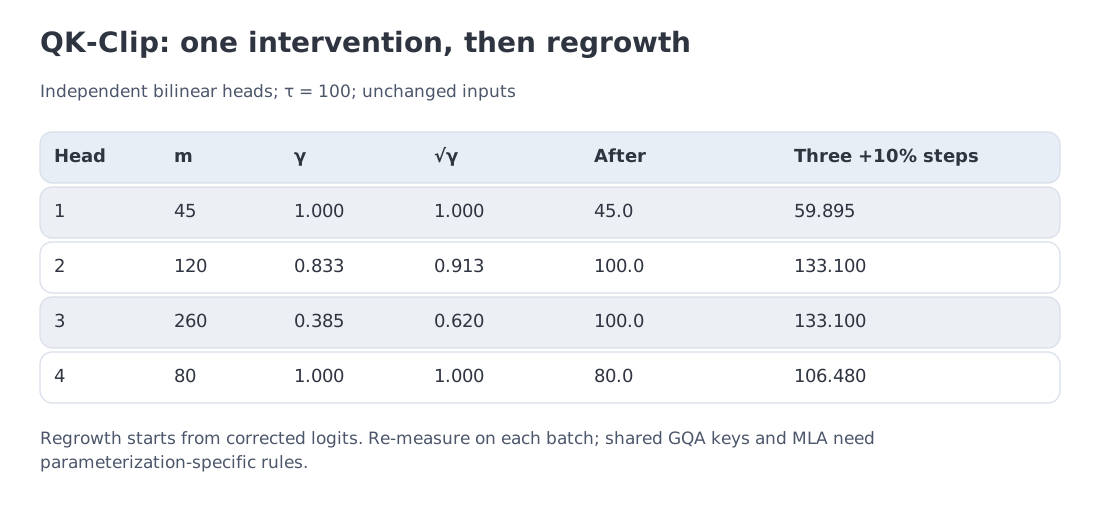 Head maxima → → symmetric rescaling of and → corrected maxima. The lower strip contrasts parameter correction with one-pass logit clipping.
The next optimizer steps can grow the weights again, so QK-Clip is part of a monitoring loop rather than a permanent vaccine. The Kimi K2 report associates the mechanism with MuonClip and reports 15.5T pretraining tokens with zero loss spikes. That is a result of one documented run, not a theorem that MuonClip prevents divergence on every architecture.
The teaching example uses an ordinary MHA-like parameterization. Kimi K2 uses MLA, where the actual clipping path is more involved. The simplified trace keeps the essential bilinear scaling argument visible enough to verify by hand.
12. Code (level 1): small functions that expose their assumptions
Most equations in this module fit into a few lines of Python. That brevity is useful only if the implementation preserves the domain of the mathematics. A negative token count should not quietly produce a complex number; a zero matrix should not pass through a polar-factor routine as if it were an ordinary update.
The first function below validates positive scalar inputs. ScalingLaw keeps the fitted coefficients and the compute convention in one object. newton_schulz accepts both tall and wide matrices and makes the transpose convention explicit. qk_clip_scales computes the intervention without mutating model parameters, which makes the arithmetic independently testable.
"""Minimal mechanisms embedded verbatim in the lecture and notebook."""
from dataclasses import dataclass
import math
from numbers import Real
import numpy as np

def positive(name, value):
    if isinstance(value, (bool, np.bool_)) or not isinstance(value, Real):
        raise ValueError(f"{name} must be a real number")
    value = float(value)
    if not math.isfinite(value) or value <= 0:
        raise ValueError(f"{name} must be positive and finite")
    return value

@dataclass(frozen=True)
class ScalingLaw:
    E: float = 1.69
    A: float = 406.4
    B: float = 410.7
    alpha: float = 0.34
    beta: float = 0.28
    kappa: float = 6.0

    def __post_init__(self):
        for name in ("A", "B", "alpha", "beta", "kappa"):
            object.__setattr__(self, name, positive(name, getattr(self, name)))
        if isinstance(self.E, (bool, np.bool_)) or not isinstance(self.E, Real):
            raise ValueError("E must be a real number")
        if not math.isfinite(self.E) or self.E < 0:
            raise ValueError("E must be finite and non-negative")
        object.__setattr__(self, "E", float(self.E))

    def loss(self, N, D):
        N, D = positive("N", N), positive("D", D)
        return self.E + self.A * N**(-self.alpha) + self.B * D**(-self.beta)

    def optimal_split(self, C):
        C = positive("C", C)
        N = (
            (self.alpha * self.A) / (self.beta * self.B)
            * (C / self.kappa) ** self.beta
        ) ** (1 / (self.alpha + self.beta))
        return N, C / (self.kappa * N)

def newton_schulz(G, quintic_steps=5):
    """Trace a rectangular polar-factor approximation."""
    X = np.asarray(G, dtype=np.float64)
    if X.ndim != 2 or 0 in X.shape or not np.isfinite(X).all():
        raise ValueError("G must be a finite non-empty matrix")
    if isinstance(quintic_steps, bool) or not isinstance(quintic_steps, int) or quintic_steps < 0:
        raise ValueError("quintic_steps must be a non-negative integer")
    scale = np.max(np.abs(X))
    if scale == 0:
        raise ValueError("G must not be all zeros")
    transposed = X.shape[0] > X.shape[1]
    X = (X.T if transposed else X) / scale
    X /= np.linalg.norm(X, ord="fro")
    for _ in range(quintic_steps):
        XXt = X @ X.T
        X = 3.4445 * X - 4.7750 * XXt @ X + 2.0315 * XXt @ XXt @ X
    return X.T if transposed else X

def qk_clip_scales(max_logits, tau=100.0, split=0.5):
    """Return gamma and Q/K scales for one monitoring step."""
    maxima = np.asarray(max_logits, dtype=np.float64)
    if maxima.ndim != 1 or maxima.size == 0 or not np.isfinite(maxima).all():
        raise ValueError("max_logits must be a finite vector")
    if np.any(maxima < 0) or not 0 <= split <= 1:
        raise ValueError("maxima must be non-negative and split must lie in [0, 1]")
    tau = positive("tau", tau)
    gamma = np.ones_like(maxima)
    over = maxima > tau
    gamma[over] = tau / maxima[over]
    q_scale = gamma**split
    k_scale = gamma**(1 - split)
    return gamma, q_scale, k_scale, maxima * q_scale * k_scale
These are diagnostic primitives, not production optimizer implementations. A complete Muon stack needs parameter groups, momentum buffers, weight decay, distributed state, mixed precision, and a policy for tensors that should remain on AdamW. A complete QK-Clip implementation must collect the appropriate statistics for the model’s attention parameterization and apply the scales to the actual parameters.
One temporal detail matters as well. The returned Q/K scales correct the state observed at the current monitoring step. Subsequent optimizer updates can enlarge the weights again. QK-Clip therefore belongs to a feedback loop: observe, intervene when necessary, and continue observing.
14. µP and MetaP: make small-model tuning informative
Suppose the target model has 100B parameters and the learning rate is still unknown. A sweep that would be routine on a 100M proxy is financially absurd at the target scale. The obvious plan is to tune the small model and reuse the result. Standard parameterization makes that plan unreliable because width changes activation scales, gradient scales, and the relative size of updates across parameter classes.
Maximal Update Parametrization (µP) addresses this transfer problem by choosing width-dependent initialization and learning-rate rules that preserve a nontrivial limiting training dynamics as width grows. When the proxy and target belong to a correctly constructed µP family, useful hyperparameters can transfer across widths far better than under standard parameterization.
The phrase “correctly constructed” carries most of the engineering burden. The two models must share the relevant architectural structure, tensors must be classified into the proper parameter types, and each type must follow its prescribed scaling rule. µTransfer is not a license to tune an arbitrary small dense Transformer and copy every value into a differently structured MoE.
The payoff is nevertheless substantial. A broad search can happen on cheap proxies; the target-scale run becomes a transfer validation rather than a fresh grid search. Scaling laws and µP solve different questions in the same planning loop. Scaling laws estimate how much model and data to buy. µP-like schemes reduce the cost of discovering how to train the selected configuration.
Meta has described MetaP in the public account of Llama 4 as a related transfer technique for critical quantities such as per-layer learning rates and initialization scales across changes in width, depth, batch size, and training-token count. The public description is less formal than the µP theory, so it is safest to treat MetaP as a method with a closely related engineering objective rather than as a synonym for µP.
15. Parallelism: fitting the training state before optimizing communication
A perfect corpus and optimizer are irrelevant if the training state does not fit in memory. Start with a deliberately simple mixed-precision AdamW accounting:
- bf16 parameter: 2 bytes;
- bf16 gradient: 2 bytes;
- fp32 master parameter: 4 bytes;
- first moment : 4 bytes;
- second moment : 4 bytes.
That is 16 bytes per parameter, before activations, temporary buffers, communication workspaces, allocator fragmentation, or checkpoint staging. A 7B model therefore requires
per fully replicated data-parallel rank. Adding GPUs increases aggregate throughput but does not reduce this replicated payload.
A distributed process is called a rank; the example maps one rank to one device. ZeRO means Zero Redundancy Optimizer; FSDP, Fully Sharded Data Parallel, denotes implementations that distribute parameters, gradients, and optimizer state. A recipe that stores gradients in fp32 needs a different byte accounting from the 16-byte policy here.
ZeRO and FSDP: shard duplicated state
ZeRO removes duplication in stages: optimizer state first, then gradients, then parameters. Under an idealized ZeRO-3 split across 64 ranks, the listed 112 GB becomes
This is a lower bound for the enumerated state, not a promise about peak device memory. Real training still needs activations, gathered parameter windows, communication buffers, and working space. The arithmetic nevertheless captures the central idea: the data-parallel group becomes a memory resource, not only a throughput resource.
Tensor parallelism: split one layer’s matrices
When a layer is itself too large or its compute needs to be distributed, tensor parallelism partitions projections by rows or columns and combines partial results with collective communication. It is most attractive inside a node or another domain with very high interconnect bandwidth. Across a slower fabric, collective latency and traffic can dominate the saved compute.
Pipeline parallelism: split the network by depth
Pipeline parallelism assigns groups of layers to stages. Its characteristic cost is idle time while the pipeline fills and drains. For balanced 1F1B (one forward, one backward) stages with communication time omitted, the bubble fraction is
where is the number of stages and the number of microbatches. With and ,
Increasing the microbatch count to 128 gives
More microbatches amortize filling and draining the pipeline. With local microbatch size fixed, they also enlarge the global batch per optimizer step. In 1F1B, the number of live activation sets is bounded by pipeline depth once the steady schedule is reached; it need not grow linearly with the microbatch count. GPipe, which accumulates all forward passes before backward passes, has different activation storage requirements.
Expert parallelism: place sparse capacity
MoE adds a different partitioning problem. The full parameter set is large, but only a subset of experts is active for a token. Expert parallelism places experts across devices and routes token representations to them. Its limiting resource may be all-to-all communication and load balance rather than matrix size alone.
Frontier runs combine these axes: data or FSDP sharding, tensor parallelism, pipeline parallelism, context parallelism for long sequences, and expert parallelism for MoE. The correct combination follows the topology. A parallelism plan that is efficient on an NVSwitch island can become communication-bound when the same collectives cross racks.
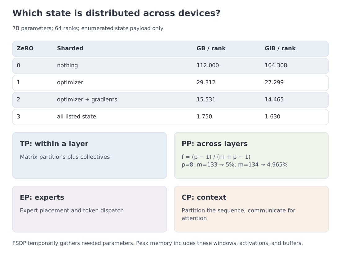 The memory and parallelism ladder: replicated AdamW state, ideal ZeRO-3/64, tensor partitioning, a pipeline with its 1F1B bubble, expert placement, and a combined frontier-scale layout.
Distributed training deserves its own course. The next layer includes topology-aware placement, context parallelism, bidirectional pipeline schedules, NCCL/RCCL behavior, asynchronous checkpointing, fault recovery, silent data corruption, and elastic response to failed nodes. The arithmetic here is enough to read a training passport and to understand why a run combines several forms of parallelism; it is not a substitute for operating a 10,000-GPU cluster.
16. Four directions in contemporary pretraining
A list of isolated tricks hides the larger pattern. Recent pretraining systems have been changing four parts of the training problem: the data schedule, the route to long context, the density of the learning signal, and the numerical representation of the run.
16.1. Data is scheduled, not merely sampled
A training mixture is no longer necessarily fixed from the first token to the last. Teams can change domain weights, increase the share of highly filtered material near the end, or use a proxy model to optimize the mixture. Curriculum and annealing turn ordering into a hyperparameter.
DoReMi makes the domain weights themselves an optimization problem. Synthetic textbook-like material and rewritten web documents attempt to improve the quality of a limited raw source rather than only enlarging it. Reasoning traces and formal material can also appear before post-training, shaping the base model toward the kinds of structure later reinforced by SFT or RL.
16.2. Long context is often a staged capability
Training the entire base run at extreme sequence length is expensive and may waste compute before the model has learned basic syntax, knowledge, and local dependencies. A common pattern is a shorter-context base phase followed by continued training or specialized extension at longer lengths. Meta describes Scout as pretrained and post-trained at 256K before generalizing to 10M; a final context limit does not mean every pretraining example used that length. The exact recipe depends on the attention architecture and positional scheme, but the economic motivation is stable: pay the long-context cost when the model can benefit from it.
16.3. One forward pass can carry a denser target
Multi-token prediction adds auxiliary heads that predict several future tokens, increasing the supervision extracted from each hidden state and potentially supporting speculative decoding later. Meta reports co-distilling Maverick from Behemoth. Distillation also moves earlier in the lifecycle: a larger family member can shape a smaller sibling during or around pretraining, rather than serving only as a post-training teacher.
These methods do not create information from nothing. They change how strongly and how early the available information constrains the model.
16.4. Number format has become part of the algorithm
FP8 established low-precision training as a mainstream systems choice on Hopper-era hardware. Blackwell-era NVFP4 pushes precision lower and therefore requires tighter control of scaling, calibration, accumulation, and outliers. A public run such as Nemotron 3 Ultra is valuable not merely because it names a four-bit format, but because its report documents both the recipe and the numerical failure modes encountered during the run.
A low-precision result should be read with three questions: which tensors use the format, where accumulation happens, and whether the reported gain is a throughput measurement under a specified setup or only a storage/operation-count argument. Precision is now part of optimizer and kernel design, not a serialization detail added after training.
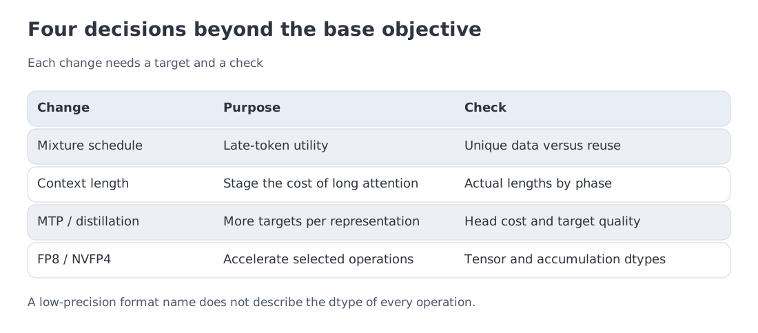 Four coordinated changes: scheduled data, staged context extension, denser learning signals, and numerical formats treated as part of the training algorithm.
17. Run passports: how to read public evidence
A model announcement tells us what can be used. A training passport tells us what was actually learned from the run. A useful passport records at least total and active parameters, token count and mixture, optimizer policy, numerical format, context schedule, parallelism, stability interventions, and the status of the evidence.
The examples below are not a leaderboard. They illustrate different degrees of transparency and different answers to the three questions that opened the module.
Kimi K2: optimizer stability at trillion-parameter scale
Kimi K2 has 1T total parameters and 32B active parameters. Its technical report describes a 15.5T-token pretraining run with MuonClip and reports zero loss spikes. The evidence matters because it connects a matrix-oriented optimizer and an explicit attention-logit control mechanism to one very large documented run.
The claim should remain scoped to that run. It does not establish that MuonClip guarantees stability for every architecture, data mixture, or hardware stack.
Nemotron 3 Ultra: low precision with a failure log
Nemotron 3 Ultra reports 550B total and 55B active parameters and 20T text tokens. Its distinguishing systems choice is NVFP4 pretraining. The report also discusses numerical incidents and the controls used to recover or prevent them.
The report describes two-dimensional block scaling, stochastic rounding, randomized Hadamard transforms, and sensitive operations kept at higher precision. BF16 branches at 5T, 10T, and 16T tokens showed an average relative training-loss gap below 0.4%. Around 8T, lowering local output-gradient accumulation from FP32 to BF16 caused instability; rolling back and restoring FP32 stabilized the run. The second divergence near 16T was not resolved by switching everything to BF16; its cause remained undetermined, and earlier learning-rate decay mitigated it.
That failure record is scientifically useful. A polished final loss curve alone cannot tell an engineer which tensors were sensitive, how scaling was managed, or where four-bit training departed from an FP8 recipe.
DeepSeek V4: one stack, several coupled innovations
The first DeepSeek V4 technical report describes the Pro model at 1.6T total and 49B active parameters and a smaller Flash model at 284B total and 13B active. The family combines hybrid attention, mHC residual connections, Muon, and more than 32T training tokens. mHC (Manifold-Constrained Hyper-Connections) extends a residual stream into interacting channels and constrains their mixing matrices. The Birkhoff-polytope structure restricts mixing to a doubly stochastic form, helping control signal amplification; a stable component in one architecture does not establish transfer to every other family. Module 6 supplies the residual-path background.
Here the lesson is coupling: attention geometry, residual transport, optimizer behavior, and data scale are parts of one system rather than independent switches.
The report’s first version is dated 26 April 2026. NIST CAISI published an evaluation of DeepSeek V4 Pro on 1 May 2026. The two sources answer different questions: the technical report documents the developer’s architecture and run; the external evaluation studies model behavior under its own protocol.
Kimi K3: scale, long context, and a more structured MoE
Kimi K3 was released with a technical report and full weights on 27 July 2026. The model has 2.8T total parameters and 104B active parameters, supports a 1M-token context, and uses architectural components including Kimi Delta Attention, Attention Residuals, and a Stable LatentMoE design with 16 active experts out of 896. The report also describes head-wise Muon and a developer-reported improvement in scaling efficiency relative to K2.
The reported gain is about 2.5× within the developers' scaling comparison with K2. K3 also separates pretraining optimization from post-training quantization: QAT starts during SFT with MXFP4 weights and MXFP8 activations. Quantile Balancing controls expert load. These are different interventions, not consequences of a single optimizer choice.
The scaling gain is a result reported by the model’s developers. It is valuable evidence about their training program, but it is not an independently measured universal law.
Qwen3.8-Max: downloadable weights, incomplete run evidence
As of 11 October 2026, both the Max API and Qwen3.8-2.4T-A95B text weights are available. The checkpoint uses the qwen3.8-max license and reports 2.4T total parameters, 95B active parameters, and a 1M-token context. The API product and downloadable text model have different feature sets.
A model card still leaves substantial gaps in a reproducible training account: the data mixture, optimizer and precision policies, context schedule, and stability history need their own evidence. Developer benchmarks describe outcomes without isolating the contribution of each pretraining choice. Access, licensing, and training transparency should be recorded separately.
Inkling: multimodal scale and a hybrid optimizer policy
Thinking Machines Lab reports 975B total and 41B active parameters for Inkling and 45T multimodal training tokens. The published account describes Muon for large matrices and Adam for the remaining parameter classes, with weight decay coupled to the square of the learning rate.
This is a concrete example of a parameter-class optimizer policy. “Trained with Muon” does not imply that every tensor in the model receives the same update rule.
Llama 4 Behemoth: infrastructure evidence from a model still in progress
Meta’s Llama 4 announcement described Behemoth as a training-stage model rather than a completed public release. The infrastructure account reports FP8 training on 32K GPUs at 390 TFLOP/s per GPU and a mixture exceeding 30T tokens. It is therefore useful as evidence about training infrastructure and MetaP, but not as a completed open model passport.
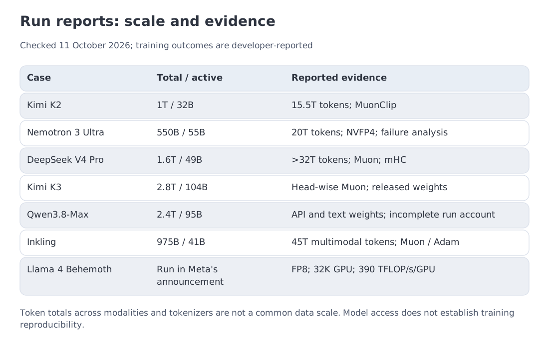 Seven public cases compared by scale, data, optimizer or numerical method, transparency, and release status. The purpose is to read evidence, not to rank model quality.
A good reading habit is to separate five verbs: measured, derived, reported, released, and planned. Many apparent contradictions disappear once each sentence uses the correct one.
20. Key takeaways and sources
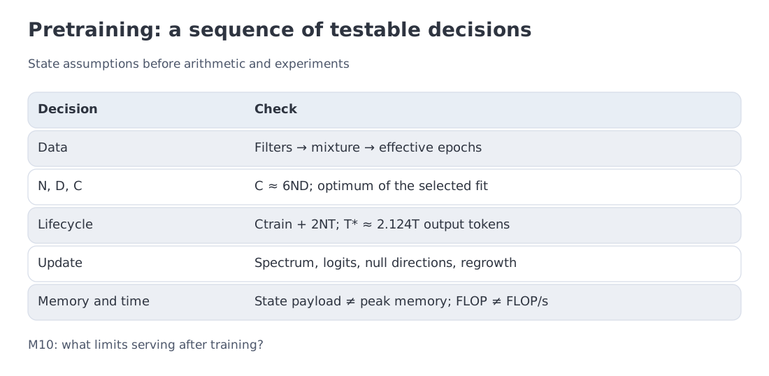 The module on one page: fitted scaling law, analytic split, inference-aware break-even, data pipeline and data wall, Muon and QK-Clip, training-state memory, parallelism, and public run passports.
A pretraining plan is a coupled decision about data, scale, and optimization.
With the fitted law
the analytic split is
The optimum is mathematically exact for the chosen approximation. Its empirical reliability depends on the fitted range, the data regime, and the objective being optimized.
Inference-aware planning changes that objective. The 8.03B/15T teaching scenario has a fitted loss 0.025804 above the same-budget optimum but a much smaller dense decoding cost. In the equal-fitted-loss comparison with a 70B model, the total-compute break-even occurs at generated tokens.
Token count alone does not describe a corpus. Extraction, language identification, heuristic cleaning, near-duplicate removal, model-based quality scoring, PII and policy filtering, domain mixture, and scheduling determine what means. As high-quality independent data becomes harder to acquire, provenance and marginal value matter more than another undifferentiated trillion-token headline.
Muon treats large updates as matrices and reshapes their singular spectrum through a short Newton–Schulz trace. QK-Clip complements that geometry by correcting parameter sources of excessive attention logits. Both mechanisms are useful only when described with their monitored quantities, parameter scope, and failure boundaries.
Memory arithmetic constrains every optimizer choice. In the module’s convention, mixed-precision AdamW state occupies 16 bytes per parameter. A 7B model therefore carries 112 GB = 104.31 GiB of fully replicated state; ideal ZeRO-3/64 reduces the enumerated payload to 1.75 GB = 1.63 GiB per rank. Tensor, pipeline, context, and expert parallelism solve different placement and communication problems.
Public training systems should be read through passports rather than slogans. Kimi K2 documents MuonClip and a 15.5T-token run; Nemotron 3 Ultra documents NVFP4 training and its numerical controls; DeepSeek V4 combines Muon, mHC, hybrid attention, and more than 32T tokens; Kimi K3 was released with full weights at 2.8T total and 104B active parameters; Inkling reports a hybrid Muon/Adam policy over 45T multimodal tokens. Qwen3.8-Max illustrates the separate axes of API access, published text weights, and incomplete pretraining disclosure.
Primary sources
- Kaplan et al., Scaling Laws for Neural Language Models
- Hoffmann et al., Training Compute-Optimal Large Language Models
- Sardana et al., inference-aware scaling
- FineWeb and FineWeb-Edu
- FineWeb2
- DCLM
- Nemotron-CC
- DoReMi
- Muon reference implementation
- Kimi K2 technical report
- µP
- ZeRO
- mHC
- DeepSeek V4 technical report
- Kimi K3 technical report, official technical blog, and full weights
- Qwen3.8-Max official announcement
- Hugging Face July 2026 incident timeline
- Nemotron 3 Ultra technical report
- Inkling official description
- Llama 4, MetaP, and FP8 infrastructure
- NIST CAISI evaluation of DeepSeek V4 Pro
Next. Module 10 moves from the cost of creating a model to the cost of serving it. KV state, memory bandwidth, batching, and cache placement will show why two models with similar parameter counts can behave very differently under a real inference workload.
Sources and access checked on 11 October 2026. Run results retain their developer-reported status; calculations from the historical fit are illustrative, not quality forecasts for current models.