Module 2. Tokenization and Embeddings
Modern LLMs · Module 2 lecture · revision 2026.10.24 · 11 October 2026
Module 1 used a document assistant to make model selection concrete. Now consider one detail of that choice: how much of a document will fit into the model's context? A published context limit counts tokens, and different models can turn the same document into different numbers of tokens. Understanding that difference requires following the interface between text and a neural network.
A tokenizer divides a string into pieces and assigns each piece an integer token ID. An embedding lookup selects a learned vector for each ID. We will trace those operations, measure the resulting sequence, and calculate the memory needed for the vector table. We will also follow the output side: a network scores candidate IDs, a generation rule selects one, and a decoder turns selected IDs back into text.
Bring Python lists, dictionaries, and functions. Section 4 explains why we use regular expressions, and Section 11 works through small matrices before discussing their memory cost. The optional learning step in §11.4 introduces the derivative and gradient needed for that calculation. Transformer architecture is not a prerequisite; Module 3 will build the network between these input and output operations.
Choose a reading route
| Pass | Route | Aim |
|---|---|---|
| First: follow the mechanism | §1 → §3 before the optional detail → §4 → §5.1–5.2 → §11.1–11.2 → §16.1; E1 and the lookup part of E6 | Distinguish bytes, token pieces, IDs, and vectors; follow one merge and one lookup |
| Second: reproduce the results | §5.3–5.4, §6–7, §11.3–11.4; notebook, E2–E3, and the learning step in E6 | Train and test BBPE, interpret measurements, calculate memory, and update a table |
| Reference: inspect real systems | §2, §8–10, §12–13, §16.2, the §3 detail; projects E4–E5 | Read tokenizer artifacts and design controlled comparisons |
On the first pass, focus on what the regex produces; its syntax can wait. Run notebook cells from top to bottom even when reading only selected explanations: later code depends on earlier definitions.
1. Follow one string into the model
Consider Привет, the Russian greeting. It contains six Unicode code points, the numeric labels used to represent its letters. UTF-8 encodes those labels as bytes. A byte is an eight-bit integer from 0 to 255; each letter in this example needs two. Our tokenizer combines selected byte sequences into larger token pieces using Byte-level Byte Pair Encoding (BBPE). Each combination of adjacent units is called a merge. Section 3 will demonstrate one merge on a short ASCII string before we trace the byte-level algorithm.
| Stage | Representation of Привет |
|---|---|
| Unicode | 6 code points |
| UTF-8 | 12 bytes: D0 9F D1 80 D0 B8 D0 B2 D0 B5 D1 82 |
| Frozen teaching BBPE, 4,096 merges | 3 IDs: [943, 370, 301] |
| Embedding table | 3 vectors: |
An ID is an index into this particular vocabulary. Its magnitude has no semantic meaning: ID 943 is not “more meaningful” than ID 370. The associated vector is learned with the neural network. In the conventional setup, the tokenizer is built separately and frozen before model training.
Replacing twelve byte positions with three token positions shortens the sequence the model processes. The tradeoff is that larger pieces need a larger inventory and a larger vector table. We will calculate both sides of that tradeoff.
Context and cost. Under one fixed input-token rate, tripling the token count triples the input-token charge and the number of context positions occupied. The factor must be measured on specified content: no universal multiplier describes the cost of a language.
Task representation. Six digits, two three-digit groups, and one token for 123456 give the network different inputs. Code indentation and function names raise the same issue. A useful segmentation can support learning; it cannot guarantee arithmetic or programming ability.
Message structure. Some IDs represent protocol markers rather than ordinary text pieces. They can delimit messages, roles, or tool calls. Section 8 explains how applications keep these markers distinct from user text.
Parameters. In the historical Llama-3.1-8B example, separate input and output tables contain parameters: about 1.05 billion, or roughly 13% of 8 billion. Section 11 explains what these two tables do and how sharing them changes the cost.
2. From word vocabularies to byte-level subwords
Early neural NLP commonly used a fixed word vocabulary and an <UNK> token. The design was simple but brittle: unseen names and misspellings became OOV—Out of Vocabulary, and morphologically rich languages produced enormous word-form inventories.
Character models reduced unknown-word problems within their chosen alphabet at the cost of much longer sequences. The useful compromise arrived through BPE—Byte Pair Encoding. Philip Gage introduced BPE as a data-compression algorithm in 1994; Sennrich, Haddow, and Birch adapted repeated pair merging to neural machine translation in 2015. Frequent strings become single symbols, while rare strings remain decomposable.
SentencePiece made subword training independent of language-specific whitespace tokenizers. It supports both BPE and a Unigram model, which chooses segmentations using piece probabilities and represents spaces explicitly, usually with ▁. SentencePiece appears in T5, Llama 1/2, Gemma, and many other open families. Architectural ancestry does not prove that a closed service uses the same tokenizer artifact, so Gemini should not simply be inferred from Gemma.
GPT-2 took another step: BBPE—Byte-level Byte Pair Encoding begins with the 256 possible bytes rather than Unicode characters. Any UTF-8 string is representable without <UNK>. The tradeoff is visible in the starting sequence: the Russian letters used below take two bytes each, and many emoji take four. Training merges frequent adjacent byte sequences. A learned piece may be a character, a word fragment, or a sequence crossing a character boundary; the algorithm imposes no character-to-morpheme hierarchy.
OpenAI’s public tiktoken family grew from r50k_base to cl100k_base and then o200k_base. A larger vocabulary can shorten target-domain sequences, but it also enlarges embeddings and creates more rows that must receive enough training signal.
In August 2025, the open gpt-oss release introduced the Harmony response format and the o200k_harmony encoding. Harmony reuses o200k_base content ranks and adds a large special-ID range for messages, channels, calls, and future protocol extensions. The official mapping in tiktoken assigns gpt-oss-* to o200k_harmony; gpt-5-* remains mapped to o200k_base.
A separate research branch avoids a fixed subword vocabulary. MEGABYTE, MambaByte, Byte Latent Transformer, and related systems model bytes or form dynamic patches. The published configurations in §9 still allocate a fixed vocabulary. Changing the input representation affects stored attention states (the KV cache), reuse of computation for repeated prompts, and generation algorithms. Later modules explain these systems in detail.
3. Compressing a sequence
Start with an ASCII example: in ababab, the adjacent pair a,b occurs three times. Replacing its non-overlapping occurrences with a new token ab turns six units into three. This is one step of BPE—Byte Pair Encoding, which repeatedly merges adjacent pairs.
For a corpus, the average number of input bytes covered by one token is
On fixed text, a higher value means a shorter model sequence. The ASCII example moves from 1 to 2 bytes/token. A bit-level compression calculation needs one more ingredient: how many bits represent an ID?
Suppose IDs lie in the range through . A fixed-width representation requires bits per ID, giving
For dense IDs, equals the number of vocabulary entries. Holes make those quantities different (§9). A complete archive must also store the vocabulary, merge rules, and metadata. LLM engineering usually cares first about shortening the sequence the network processes.
Optional detail: distribution mismatch and the word2vec connection
If a source emits with probability but a probabilistic code uses , its ideal expected length is
is source entropy in bits. KL divergence measures the extra cost of mismatched probabilities, assuming wherever . Deterministic BPE is not arithmetic coding under a probability model, so a bytes/token difference is not a KL estimate. The RU-train/EN-evaluation comparison in §5 changes language and training exposure together; the separate RU evaluation partition provides a control.
After §11, another connection becomes useful. SGNS, skip-gram with negative sampling, can be interpreted as implicitly factorizing a shifted PMI—Pointwise Mutual Information matrix:
Here is a word, a context, and the number of negative samples. The per-dot-product optimum comes from an idealized SGNS analysis with negatives drawn from the context distribution; finite vector dimension and different negative sampling distributions change the result. GloVe uses a separate explicit objective on co-occurrence statistics. Transformer embeddings retain the ID-to-vector interface, but their training objective does not require this PMI factorization.
Information Theory for ML, Modules 2 and 6, develops the coding theory. The practical lesson here is that the usefulness of a representation depends on the data distribution.
4. The tokenizer as a sequence of operations
encode(s) returns integer IDs. decode(ids) joins the byte pieces assigned to those IDs and reads the result as text. Let be the set of defined IDs: an encoded sequence is with , where is its length. Our BBPE maps the empty string to an empty list.
The teaching implementation preserves text exactly:
provided is representable as valid UTF-8 and no normalization changes it. Python strings containing lone Unicode surrogates are outside this domain; encoding rejects them.
Normalization transforms input before segmentation. It may map full-width letters to ordinary letters or collapse repeated spaces. If the normalizer is , complete vocabulary coverage allows recovery of , which need not equal . SentencePiece defaults to nmt_nfkc and removal of extra spaces. An unknown-token replacement can lose even normalized content, so round-trip claims need a specified configuration.
Step 0. Pre-tokenization
A regular expression divides the input into chunks, the regions within which merging is allowed. The teaching PAT.findall produces:
| Input | Chunks in Python notation |
|---|---|
Hello world! | ['Hello', ' world', '!'] |
1234567 | ['123', '456', '7'] |
Привет | ['Привет'] |
The leading space belongs to world. BPE cannot merge across the boundary after Hello. Digits are grouped into at most three positions before learning begins. These constraints are an inductive bias: a deliberate restriction on the representations the algorithm can learn, not a guarantee of arithmetic ability.
Here is the full cl100k-like teaching pattern. Spaces around | are for presentation only; §6 contains the executable form without them.
'(?i:[sdmt]|ll|ve|re) | [^\r\n\p{L}\p{N}]?+\p{L}+ | \p{N}{1,3} | ?[^\s\p{L}\p{N}]++[\r\n]* | \s*[\r\n] | \s+(?!\S) | \s+
The branches handle English contractions, letters with an optional leading character, digit groups, punctuation, and whitespace. The actual o200k_base pattern is more elaborate; this implementation does not claim bit-exact compatibility.
Step 1. BPE training
Convert each chunk to bytes. At each training step select the most frequent adjacent pair:
Replace its non-overlapping occurrences with a new ID whose byte piece concatenates the pieces for and . Our implementation breaks frequency ties by first encounter. That choice affects every later merge and is part of the specification.
When each step adds one ID and special IDs are disjoint from ordinary ones, the number of defined IDs is
Special-token names can outnumber their IDs. The model's allocated vocabulary dimension can also exceed . Sections 8–9 separate these quantities.
Step 2. Encoding new text
Apply the same chunking and byte conversion. A merge's rank is its priority in the learned ordered list. Repeatedly merge the present pair with the smallest rank, stopping when no learned pair remains. Encoding does not train on the new string or recount corpus frequencies. In our format, new IDs 256,257,… also specify merge order.
Step 3. Decoding and measurement
Decode joins token bytes before interpreting UTF-8. One token may contain only part of a character, so a streaming decoder must buffer an unfinished byte suffix. Replacing invalid bytes with � is a display policy that loses information.
The byte alphabet covers any valid UTF-8 input without <UNK>, even when every byte remains separate. Measure efficiency on named data: bytes/token counts bytes per token; chars/token here counts Unicode code points; fertility counts tokens per word; single-token retention measures the fraction of selected words represented by one token. The last two require a word definition and a policy for leading spaces.
5. Worked example: from UTF-8 to a compression curve
The complete path is shown first.
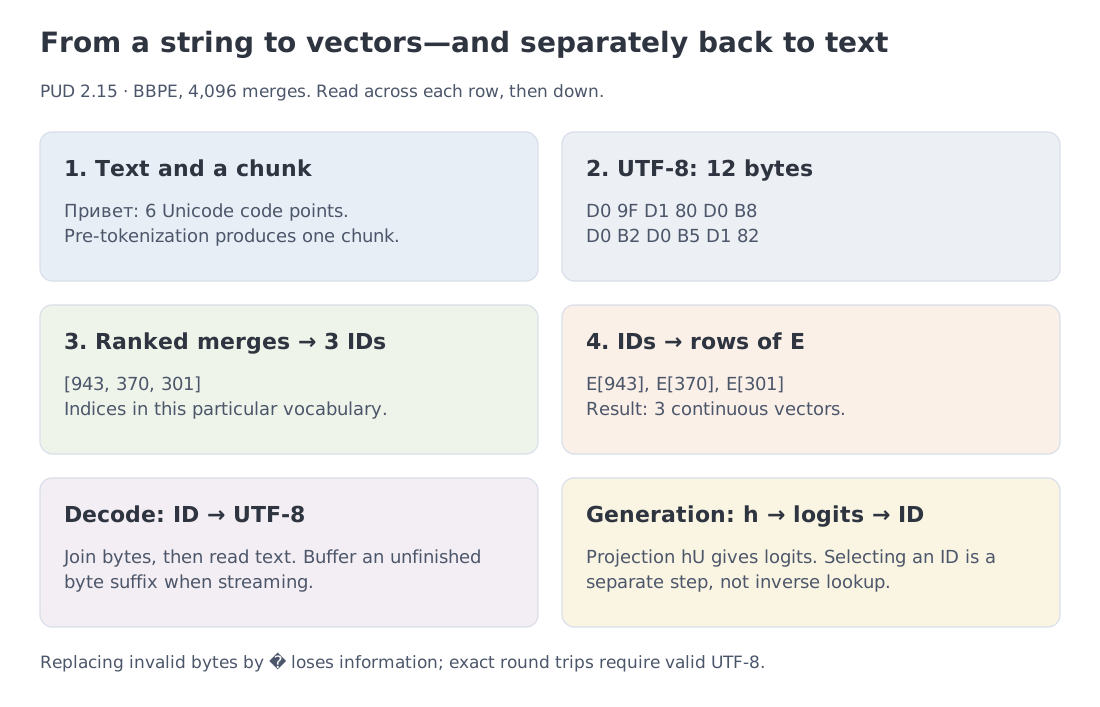 Text is pre-tokenized, encoded as UTF-8 bytes, merged by rank, mapped to IDs, and looked up in the embedding table.
5.1. The byte starting point
| String | Code points | UTF-8 bytes | Hex bytes |
|---|---|---|---|
Привет | 6 | 12 | D0 9F D1 80 D0 B8 D0 B2 D0 B5 D1 82 |
é | 1 | 2 | C3 A9 |
🚀 | 1 | 4 | F0 9F 9A 80 |
ток | 3 | 6 | D1 82 D0 BE D0 BA |
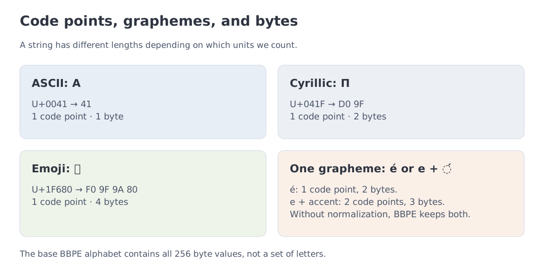 In these examples, П occupies two bytes, 🚀 four, and ASCII A one. Other emoji and visible characters can contain multiple code points. BBPE starts from bytes.
Before merges, Hello has five byte tokens and Привет has twelve. Vocabulary training can reduce the gap, but the byte representation determines the starting point.
A code point is not always a visible character. é is one code point, while the similar-looking e\u0301 is two—a letter and a combining accent—but one grapheme. Our BBPE does not normalize these spellings; their distinct byte sequences are preserved.
5.2. Six visible merge steps
The toy corpus is низко низко летали ласточки, ласточки летали низко, totaling 93 bytes after chunking. The first six merges are:
| Step | Pair | Count | Resulting fragment |
|---|---|---|---|
| 1 | D0 + B8 | 7 | Cyrillic и |
| 2 | space + D0 | 6 | space plus first Cyrillic byte |
| 3 | D0 + BA | 5 | к |
| 4 | D0 + BE | 5 | о |
| 5 | (space+D0) + BB | 4 | ' л' |
| 6 | ' л' + D0 | 4 | prefix of a longer fragment |
After six merges, 93 bytes become 62 tokens. The first merge forms the letter «и», but the second joins a space to the first byte of a Cyrillic letter. Frequency, rather than a linguistic hierarchy, determines which piece appears next. Intermediate symbols remain in the vocabulary even when longer merges later make them rare.
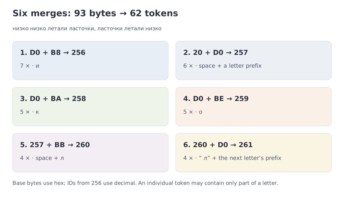 The toy trace moves from raw bytes to Cyrillic characters and a leading-space fragment.
5.3. Separate training exposure from language
Our external text comes from Parallel Universal Dependencies (PUD), UD release 2.15: aligned translations of news and Wikipedia sentences. The course includes a fixed local copy. The corpus record provides both upstream commits, SHA-256 hashes, extraction rules, and CC BY-SA 3.0 attribution. Notebook execution does not download the corpus.
Partition entire source documents together in both languages. Training contains 833 sentence pairs from 331 documents; evaluation contains 167 pairs from 66 other documents. BBPE sees only the 180,112-byte Russian training text. The parallel evaluation texts contain 33,654 Russian bytes and 18,168 English bytes. These counts include LF sentence separators and a final LF. This is a teaching partition for tokenization; upstream PUD is a parsing test set. PUD counts aligned segments, occasionally containing two grammatical sentences. Most source texts were originally English; translation history and topic selection limit broader language claims.
| Merges | RU train bytes/token | RU evaluation bytes/token | EN evaluation bytes/token | RU phrase tokens | EN phrase tokens |
|---|---|---|---|---|---|
| 0 | 1.000 | 1.000 | 1.000 | 61 | 26 |
| 64 | 2.236 | 2.244 | 1.009 | 35 | 26 |
| 256 | 3.231 | 3.213 | 1.011 | 19 | 26 |
| 1024 | 4.531 | 4.360 | 1.047 | 15 | 26 |
| 4096 | 6.535 | 5.542 | 1.317 | 13 | 22 |
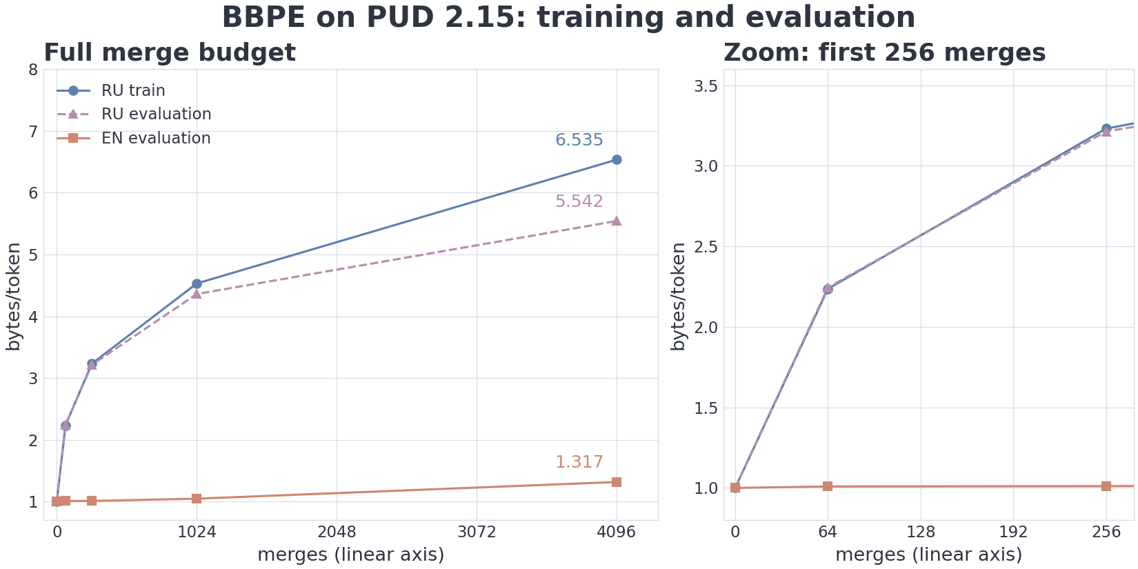 One RU-trained tokenizer applied to three partitions. The Russian evaluation set contains unseen documents; the English set contains the aligned translations of those same evaluation sentences.
At 4,096 merges the training text reaches 6.535 bytes/token, compared with 5.542 on new Russian documents. This is a result for these partitions, not a population-wide estimate of overfitting. English evaluation reaches 1.317: a vocabulary learned from Russian leaves much of this English text in small byte-level pieces.
The parallel evaluation sets control content and training exposure more closely than RU-train versus EN-evaluation. However, bytes/token still depends on UTF-8: a higher byte count per token does not establish a lower cost for equivalent content. Encoding each of the 167 aligned sentences separately, without an added LF, gives 6,079 RU tokens and 13,789 EN tokens, or means of 36.40 and 82.57. This compares equivalent content under one vocabulary. Do not derive it by subtracting separators from the earlier table: adding LF can change chunk boundaries and merges at the end of a sentence. To investigate the effect of training language, repeat training on EN and evaluate both languages; the matching EN training data are included.
The phrase columns use Внимание — это всё, что вам нужно. and Attention is all you need.. These are short probes, separate from the parallel evaluation. Later rules produce smaller reductions per added merge; read that change against the linear merge-count axis.
5.4. Four strings, one tokenizer
| Example | Tokens | Letter/digit runs | Fertility | Bytes/token |
|---|---|---|---|---|
| Russian prose | 16 | 7 | 2.29 | 6.94 |
| English prose | 44 | 8 | 5.50 | 1.18 |
| Python | 63 | 13 | 4.85 | 1.08 |
| Numbers and dates | 29 | 6 | 4.83 | 1.03 |
Each category contains one string, so this is not a domain ranking. Here a “word” is a match of \p{L}+|\p{N}+: a run of letters or digits, including the pieces of a date. Digit grouping, separators, and training data all affect the observed ratios; the table alone does not isolate their effects.
The exact strings (\n denotes a newline in the Python example):
Языковые модели предсказывают следующий токен по контексту.Language models predict the next token from context.def encode(text):\n return [merges.get(p, p) for p in pairs(text)]1234 + 5678 = 6912; 2026-07-04
6. Level-1 code: a transparent BBPE trainer
The algorithm needs one representation of its current state: ids is a list of chunks, each of which is a list of integer IDs. Keeping the chunks separate prevents a merge from crossing a pre-tokenization boundary.
Read the three functions as one loop. get_stats counts adjacent pairs, merge replaces non-overlapping occurrences of a selected pair, and train_bbpe repeatedly chooses and applies a rule. New IDs begin at 256 because 0–255 already represent individual bytes. The regex is the teaching specification used throughout this module; another tokenizer may impose different boundaries.
import regex as re
from collections import Counter

PAT = re.compile(
    r"""'(?i:[sdmt]|ll|ve|re)|[^\r\n\p{L}\p{N}]?+\p{L}+|\p{N}{1,3}| ?[^\s\p{L}\p{N}]++[\r\n]*|\s*[\r\n]|\s+(?!\S)|\s+"""
)

def get_stats(ids):
    counts = Counter()
    for chunk in ids:
        for pair in zip(chunk[:-1], chunk[1:]):
            counts[pair] += 1
    return counts

def merge(ids, pair, new_id):
    result = []
    for chunk in ids:
        merged, i = [], 0
        while i < len(chunk):
            if i + 1 < len(chunk) and (chunk[i], chunk[i + 1]) == pair:
                merged.append(new_id)
                i += 2
            else:
                merged.append(chunk[i])
                i += 1
        result.append(merged)
    return result

def train_bbpe(text, num_merges=1000):
    if type(num_merges) is not int or num_merges < 0:
        raise ValueError("num_merges must be a non-negative integer")
    chunks = re.findall(PAT, text)
    ids = [list(chunk.encode("utf-8")) for chunk in chunks]
    merges = {}
    for i in range(num_merges):
        stats = get_stats(ids)
        if not stats:
            break
        pair = max(stats, key=stats.get)
        ids = merge(ids, pair, 256 + i)
        merges[pair] = 256 + i
    return merges
The returned dictionary records each pair and its new ID in learning order. On the §5.2 corpus, six iterations should recover the displayed merge list and leave 62 tokens. Notice the distinction between counting and replacing: zip counts adjacent pairs even when they overlap, whereas merge consumes two elements at a time after a match. An input element can participate in only one replacement during that step.
The naive trainer rescans the corpus at every step, so its cost is . Industrial trainers update pair statistics incrementally. Equal-frequency pairs are resolved by first encounter, a rule called a tie-break. Both scanning order and replacement behavior are part of the specification. The notebook speeds up repeated chunks while explicitly checking that these choices still produce the same result.
8. Reading o200k_harmony correctly
8.1. Pre-tokenization is part of the format
The teaching regex illustrates the design space, but o200k_base uses a distinct, more detailed Unicode pattern. It has multiple letter branches for case structure and its own whitespace behavior. Harmony inherits the o200k_base pattern and mergeable ranks unchanged.
This distinction is operationally important: a tokenizer is not only a vocabulary size and merge table. The regex determines which merges are even possible.
8.2. Names, IDs, and one alias
A .tiktoken file stores base64(token_bytes) rank. In the public implementation:
o200k_baseprovides 199,998 mergeable IDs numbered0…199997;- Harmony exposes 1,091 special-token names;
- those names map to 1,090 unique special IDs;
- ten names have current protocol meanings;
- 1,081 names are spelled as reserved entries;
<|endofprompt|>and<|reserved_200018|>are aliases for ID 200018.
Therefore,
unique IDs. An alias is a second name for an existing ID. Counting the set of mapping values therefore gives one fewer item than counting names.
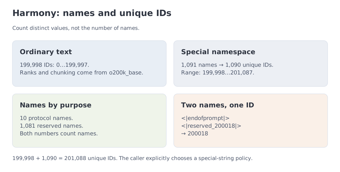 Harmony contains 199,998 mergeable IDs and 1,090 unique special IDs represented by 1,091 names.
8.3. Special-token policy is explicit
tiktoken.Encoding.encode() rejects registered special-token spellings by default. A caller must choose one of three behaviors:
- authorize selected spellings with
allowed_special; - disable the rejection with
disallowed_special=()and treat them as ordinary text; - use
encode_ordinary().
Thus a literal <|start|> neither silently becomes a control ID nor necessarily passes as ordinary text. The API call defines the boundary.
8.4. Hugging Face artifacts
A BPE tokenizer.json typically contains model.vocab, model.merges, pre-tokenizer configuration, and added tokens. tokenizer_config.json may also contain a Jinja chat template. The template inserts protocol structure around messages; it builds on the tokenizer but is a separate layer discussed in Module 13.
9. Three vocabulary sizes that answer different questions
“Vocabulary size” can refer to three quantities. Keep them separate when inspecting files or estimating memory:
- : the number of defined unique IDs, taking the union of ordinary and special IDs.
- : the ID range starting at zero, including holes.
- : the model's allocated vocabulary dimension, normally
vocab_size, which sets the input table's row count and the output score count. Direct indexing requires .
| Exact artifact | Ordinary IDs | Additional unique IDs | Model | ||
|---|---|---|---|---|---|
o200k_base | 199,998 | 2 | 200,000 | 200,019 | not established by the tokenizer |
o200k_harmony / gpt-oss-120b | 199,998 | 1,090 | 201,088 | 201,088 | 201,088 |
Qwen/Qwen3-8B | 151,643 | 26 | 151,669 | 151,669 | 151,936 |
The two o200k_base special IDs are 199999 and 200018, leaving 19 holes in the range. tiktoken.n_vocab reports , not . Qwen3-8B allocates 267 more rows than its tokenizer defines unique IDs. Extra rows are not automatically decodable tokens and do not, by themselves, establish a protocol purpose. If such positions appear in the output, generation needs an explicit policy for their eligibility. See the n_vocab implementation and Qwen3-8B config.
The next table compares model fields only, using named variants checked on 11 October 2026. The data snapshot records immutable revisions, URLs, field paths, and SHA-256 hashes; original source files are included with the module. The examples expose different configurations rather than ranking release recency or model quality.
| Published configuration | Field | Allocated dimension |
|---|---|---|
openai/gpt-oss-120b | vocab_size | 201,088 |
deepseek-ai/DeepSeek-V4-Flash | vocab_size | 129,280 |
Qwen/Qwen3-8B | vocab_size | 151,936 |
mistralai/Mistral-Small-3.1-24B-Instruct-2503 | params.json: vocab_size | 131,072 |
moonshotai/Kimi-K3 | text_config.vocab_size | 163,840 |
zai-org/GLM-5 | vocab_size | 154,880 |
nvidia/NVIDIA-Nemotron-3-Super-120B-A12B-BF16 | vocab_size | 131,072 |
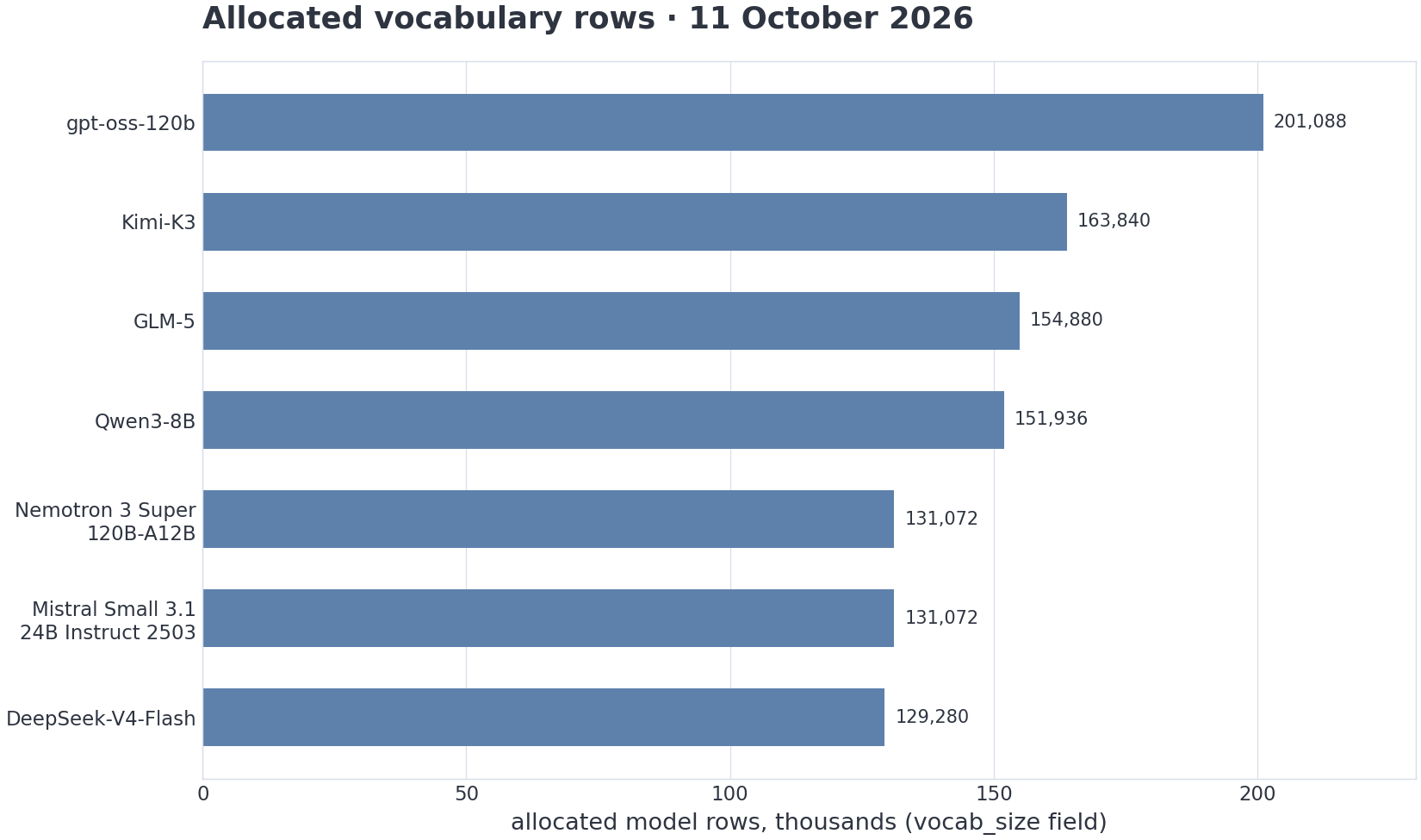 These bars show allocated model rows. They do not mix that quantity with special-token names or
tiktoken.n_vocab.
Section 11 also retains Llama-3.1-8B with as a historical memory calculation. In the pinned Transformers source, Llama4TextConfig defaults to 202048 and Gemma3TextConfig to 262208. A class default describes how a configuration object is initialized; it does not establish the contents of every released checkpoint or tokenizer file. Use the exact artifact for a model-specific calculation. Llama, Gemma, and Command A checkpoint configurations that could not be retrieved anonymously are excluded from the chart.
For Claude and Gemini, the documented interface used here is a counting API, not an inferred local vocabulary. Claude token counting returns an estimate that can differ from actual usage. Gemini countTokens likewise requires a model and request content. Gemma does not establish Gemini's vocabulary. Record the selected model, message formatting, tools, and multimodal components when counting a real request.
In research, tokenizer-free usually means no fixed subword inventory. Segmentation can still exist: BLT forms dynamic byte patches. Compare these systems by quality and the cost of the entire computational sequence.
10. Fertility, language, and domain
Fertility is tokens per word; bytes/token is source bytes per token. Both require a named evaluation corpus. Fertility additionally requires a definition of “word,” which is not neutral across writing systems. Bytes/token does not need word segmentation, but it still depends on spaces: the teaching artifact gives 1.1667 for one two and 1.1429 for one two.
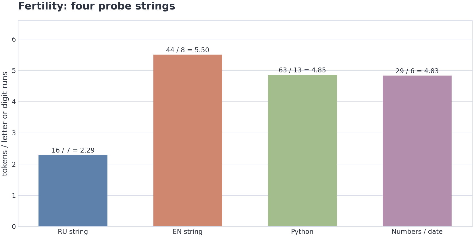 On the four individual strings in §5.4, the teaching tokenizer gives fertility 2.29, 5.50, 4.85, and 4.83 respectively.
Cross-lingual evaluation
Published studies find large token-count differences for parallel content. A defensible report records the corpus, tokenizer revision, chat formatting, word definition, and price schedule. If the same provider charges the same input rate per token, three times as many input tokens mean three times the input-token charge—not necessarily three times the entire interaction cost. Output tokens, cache hits, and tools may have different tariffs; token counts alone cannot establish the total bill or a cross-model price ranking.
Numbers
BPE and Unigram can both be deterministic once trained. They differ in how the vocabulary is learned and how segmentation is selected. Digit-group regexes reduce segmentation variability; they do not guarantee arithmetic reasoning.
Code
A code-oriented tokenizer can learn indentation patterns, operators, and frequent identifier fragments. Its benefit depends on the pretraining data as well as the vocabulary. Adding a token that rarely appears during model training creates an undertrained embedding row rather than an automatic capability.
Undertrained tokens
The tokenizer’s corpus and the model’s corpus are not always identical. Rare input IDs supply few observations for their lookup rows. With a full output softmax, all output rows generally receive gradient even when their token is not the target; rare targets provide little positive evidence, not necessarily few total updates. Poorly trained representations can result. Detecting them requires occurrence statistics and model-weight analysis, not only the merge rank.
11. Embeddings: reading an ID and predicting the next one
11.1. A lookup selects a row
Let be the model's allocated vocabulary dimension and the number of coordinates in each vector. The input table is a learned matrix . An embedding lookup for ID returns row . It neither searches for a nearby word nor multiplies a vector by the numeric ID.
Use three toy IDs and two-dimensional vectors:
Three input IDs produce a matrix . Repeated ID 0 selects the same row twice. Later network layers can produce different hidden states, or internal vectors, at those positions because their contexts differ. The input embedding and its contextual representation are distinct stages.
11.2. A projection produces scores
Take the final hidden state as a row vector . The output projection produces logits, unnormalized scores for the next ID:
Softmax turns these scores into probabilities summing to 1. Subtracting the maximum preserves the result while avoiding overflowing exponentials. This example omits an output bias, restrictions on valid IDs, and any model-specific logit transformations.
Weight tying sets . With , the table above gives and . Greedy selection chooses ID 1. Even though , the most likely output is not necessarily ID 0: the output projection does not invert the lookup.
With untied weights, is learned independently. For example,
Decoding is a separate operation on already selected IDs: join their byte pieces and interpret UTF-8. decode([943,370,301]) requires neither nor .
Practice. Notebook section 10 computes X = E[ids], both forms of h @ U, and stable softmax. It then applies one learning step and checks that repeated selections accumulate gradient into the same row. These hand-chosen matrices illustrate operations, not the semantics of a trained language model.
11.3. Parameter and memory cost
One table contains parameters. Independent input and output tables require ; tied weights require unique trainable parameters. This count omits an output bias. BF16 stores two bytes per parameter, and bytes.
| Scenario | Parameters in one table | Parameters in two tables | BF16 for two |
|---|---|---|---|
| gpt-oss-120b, | 579,133,440 | 1,158,266,880 | 2.1574 GiB |
| Llama-3.1-8B, | 525,336,576 | 1,050,673,152 | 1.9570 GiB |
| Expand exactly 100,000 → 262,000, | +663,552,000 | +1,327,104,000 | +2.4719 GiB |
The last row is a hypothetical vocabulary expansion, not a Gemma configuration. These are weight payloads only. Training also needs gradients, optimizer states, activations, and temporary buffers; weight tying alone does not determine total training memory.
The inspected gpt-oss-120b, Qwen3-8B, DeepSeek-V4-Flash, and Kimi-K3 configs set tie_word_embeddings to false. The published Gemma3TextConfig class defaults to true. Check the exact config for another model: size, API pricing, or family membership does not establish this choice.
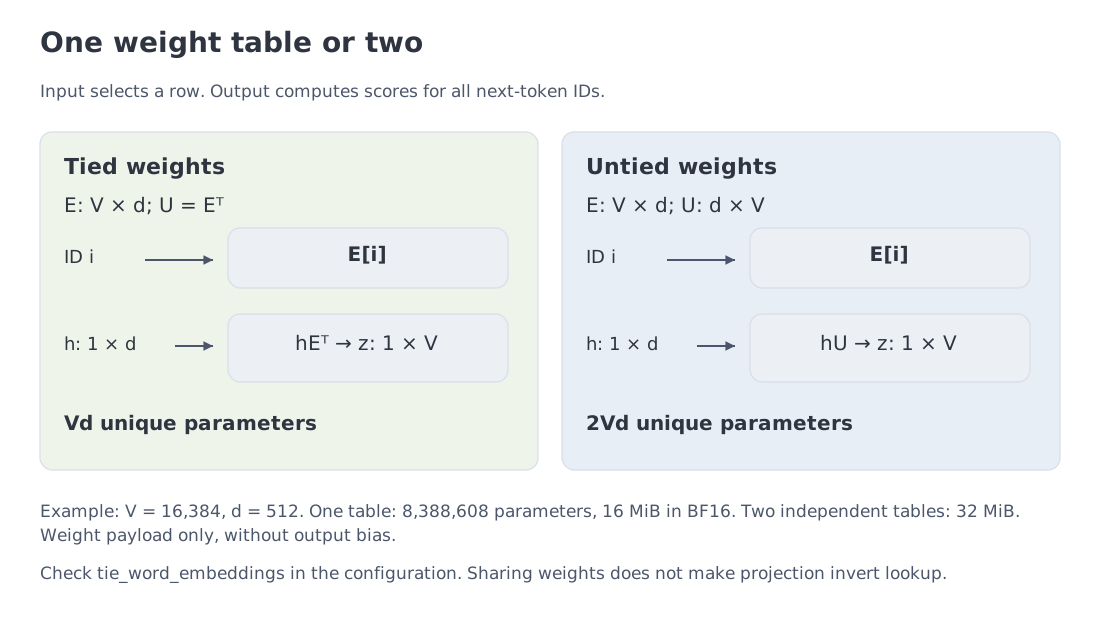 Input selects a row of E; output computes scores hU. Sharing weights saves parameters without making the operations inverses.
11.4. Updating the selected rows
Calling a learned table raises a practical question: how does selecting a row lead to changing its values? Isolate the operation with the same IDs [0,2,0]. Give each position a target vector and define
There are positions; selects a row at position , and the squared norm sums the squared coordinate differences. This loss function is smaller when the selected vectors lie closer to their targets. Zero targets make the arithmetic transparent; moving every vector toward zero is not a useful language-learning objective.
To reduce the loss, measure how it responds to a small change in each parameter. A derivative describes that local rate of change for one number. The gradient collects the derivatives for all parameters. Since the derivative of with respect to is , a selected row receives its difference from the target. Reusing the row adds another contribution:
Row 0 is selected twice, so its gradient is . Row 2 receives once. Row 1 does not enter this loss and receives zero. Thus
The learning rate sets the update size. Taking gives [[0.8,0],[2,0],[0,0.9]]. The loss falls from to . Moving a sufficiently small distance against the gradient decreases this loss; an excessively large step can increase it.
NumPy expresses the accumulation as np.add.at(grad, ids, X - targets). Every occurrence contributes, including repeated indices. In contrast, grad[ids] += X - targets operates through a temporary advanced-indexing result and does not provide that accumulation. The notebook demonstrates the difference. It also checks the derivative by finite differences: perturb one parameter slightly in each direction, measure the two losses, and divide their difference by twice the perturbation. That supplies an independent numerical check, not a practical training algorithm for a large network.
A real language model receives its signal from next-token prediction through the intervening layers. This experiment isolates the lookup table. If a shared table also participated in the output projection, its full gradient would include that path as well; our quadratic loss contains no such projection.
12. Where the token analogy extends to other modalities
A Vision Transformer (ViT) divides an image into patches, small rectangular regions, and maps each region to a vector. A vision encoder then processes the sequence. Those vectors have the vision network's feature width, which need not match the language model's width.
A connector makes the visual features compatible with the language decoder. It can change their width and may also reduce their number. Patch extraction resembles text pre-tokenization, but a typical input patch is not assigned a discrete ID from a text vocabulary. Module 16 develops the complete image-to-encoder-to-connector-to-language-model path and alternative ways to join its components.
An 896×896 image with 14×14 patches starts with regions. That is an initial patch count, not necessarily the number of language-context positions. If the resulting vectors participate in the language decoder's self-attention, they consume context positions and stored attention states, called the KV cache. Modules 3 and 5 explain those mechanisms. For now, distinguish the original image partition from the representation actually delivered to the LLM.
Neural audio codecs such as EnCodec and SoundStream use RVQ—Residual Vector Quantization. Several codebooks convert audio into discrete codec IDs and a decoder reconstructs the waveform. This is closer to text tokenization because the representation is a sequence drawn from finite codebooks.
A codebook is a finite table of vectors; quantization replaces a vector by the index of a nearby entry. Successive RVQ codebooks represent residual error. At frames/s and transmitted indices per frame, the stream contains IDs/s: 50 frames/s with 8 codebooks gives 400 IDs/s before further packing. This is an illustrative calculation, not a universal audio-model rate. Module 16 follows these representations through the audio model and distinguishes codec IDs from positions processed by the language decoder.
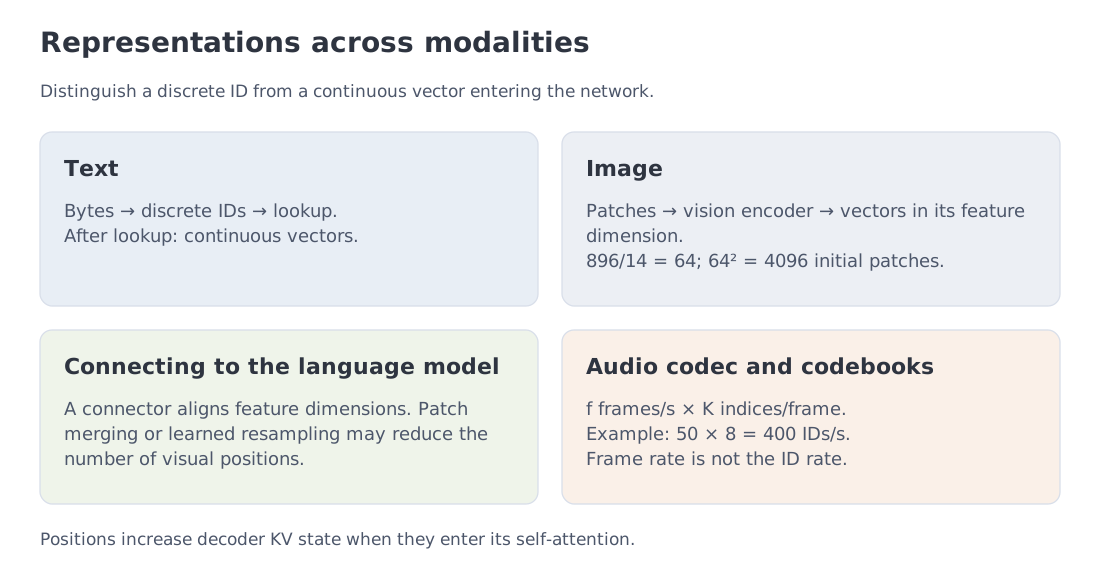 Text uses discrete subword IDs, images commonly use continuous patch embeddings, and neural codecs use discrete audio IDs.
Module 16 develops the full multimodal architecture, including connectors, dynamic image resolution, video, and streaming speech.
13. Connections to the rest of the course
We now have an input matrix and an output operation . The missing computation is how to obtain from the available context. Module 3 supplies attention and the Transformer block, showing how the same starting embedding can acquire different contextual representations.
The lookup table itself contains no position dependence. Module 4 develops explicit position and distance signals. A causal mask also constrains order by preventing access to future positions, so removing positional embeddings does not remove every source of ordering information. Module 3 makes that distinction concrete. Message templates and protocol tokens return in Module 13; visual-position and KV-memory costs appear in Modules 10 and 16; Module 11 studies efficient generation.
Further study. Source coding, KL divergence, and information-theoretic mismatch are developed in Information Theory for ML, Module 6.
16. Key takeaways
16.1. After following the mechanism
Keep the stages separate. UTF-8 represents a string as bytes. Pre-tokenization establishes the boundaries within which BPE may combine adjacent units. Training chooses frequent pairs and records their order; encoding applies those learned rules without retraining on the new string. Fewer tokens mean a shorter model sequence. Bytes/token measures that effect on specified text, while a complete storage calculation must also account for IDs and the vocabulary.
An ID indexes a row; its magnitude does not measure meaning. The input table selects a vector for each ID. The network processes context, and an output projection maps its hidden state to logits. Softmax converts those scores to probabilities. Selecting an ID and decoding selected IDs remain distinct operations. Sharing the input and output weights does not make projection an inverse lookup.
The byte alphabet covers valid UTF-8, but preserving the original spelling also requires a suitable normalization and decoding policy. Before Module 3, be able to trace string → bytes → IDs → vectors and explain separately how selected IDs become text.
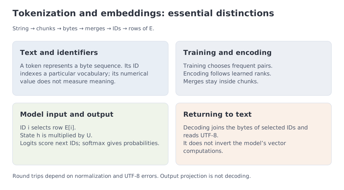 A first-pass reference: byte representation, learning and applying merges, selecting embedding rows, and decoding IDs separately.
16.2. After the experiments and artifact inspection
- Most text LLMs freeze a separately constructed tokenizer before model training. Comparisons also need the training data that determined each vocabulary.
- Compare RU train with RU evaluation, then the parallel RU/EN evaluation sets. They answer different questions; bytes/token estimates neither KL nor the cost of equivalent content.
- Harmony has 199,998 mergeable IDs and 1,090 unique special IDs represented by 1,091 names.
- Special-token interpretation is an explicit API policy.
- Defined ID count , ID range , and allocated model dimension answer different questions.
- Fertility should be paired with bytes/token and measured on fixed data.
- Weight tying saves parameters. Output projection predicts an ID; decoding maps already selected IDs to text.
- A lookup row accumulates gradient from every use. A complete language-model objective adds computational paths absent from the isolated quadratic example in §11.4.
17. Sources
Primary and technical sources:
-
Universal Dependencies PUD 2.15 — RU, EN; local provenance and attribution, CC BY-SA 3.0.
-
Gage, A New Algorithm for Data Compression — PDF
-
Sennrich, Haddow, Birch, Neural Machine Translation of Rare Words with Subword Units — arxiv.org/abs/1508.07909
-
Kudo, Richardson, SentencePiece — arxiv.org/abs/1808.06226
-
OpenAI
tiktoken— official repository -
SentencePiece normalization — documentation
-
Llama4TextConfig — source
-
Gemma3TextConfig — source
-
OpenAI Harmony — official repository
-
Petrov et al., Language Model Tokenizers Introduce Unfairness Between Languages — arxiv.org/abs/2305.15425
-
Press, Wolf, Using the Output Embedding to Improve Language Models — arxiv.org/abs/1608.05859
-
Levy, Goldberg, Neural Word Embedding as Implicit Matrix Factorization — NeurIPS 2014
-
Yu et al., MEGABYTE — arxiv.org/abs/2305.07185
-
Pagnoni et al., Byte Latent Transformer — arxiv.org/abs/2412.09871
-
Claude token-count endpoint — official documentation
-
Gemini
models.countTokens— official documentation
Next: Module 3 connects embeddings to attention, Transformer blocks, and next-token prediction. If you can already explain the complete computation, use its diagnostic to move directly to positional representations in Module 4.
Public fields and primary source files checked on 11 October 2026, with pinned revisions and SHA-256 hashes. The teaching BBPE uses the fixed external PUD 2.15 corpus. Historical calculations and configuration-class defaults are identified separately.