Module 4. Positional representations: from sinusoids to multiple axes
Modern LLMs · Module 4 lecture · 2026.10.6 edition · 10 October 2026
Module 3 explained how a query retrieves a weighted mixture of values. Here we hold the query and key content fixed and change their positions. What should happen when the tokens move together? What if the gap between them grows? Working through those questions gives us sinusoidal encoding, RoPE, context extension, and spatial or temporal coordinates for multimodal inputs.
You need dot products and the attention mechanism from M3. We will introduce rotation using a pair of coordinates; complex numbers provide an optional shorthand for the same operation.
Reading routes
- First pass: follow the geometry. Read §§1–10, using §2 as a map. The historical detail and the implementation in §4 are expandable. In §7, focus on which frequencies each method changes; return to the boundary derivation later. Finish with §§13 and 17, then try §15 without looking back.
- Implementation pass: reproduce the result. Work through the numbers in §5, the ramp in §7, and the code in §§4 and 11. Run the notebook described in §12, including its cache and precision checks, and tackle §16.
- Reference pass. Shapes and coordinate pairing: §4. Frequencies: §6. Scaling methods: §7. Configuration fields: §10. Multiple axes: §13. Verified implementation examples: §14. Module 5 then develops attention architecture and execution.
1. Motivation: content attention is not an ordering mechanism
Consider bidirectional self-attention applied to a sequence matrix , without positional information or a restrictive mask and with dropout disabled. If the rows are permuted by a permutation matrix , the result obeys
This is permutation equivariance. The output is not invariant—the rows move—but the computation has no independent way to decide that one arrangement represents “the cat chased the dog” and another represents “the dog chased the cat.” It only follows the rows it receives.
A causal mask changes the situation, because token can only attend to an allowed prefix. That asymmetry already carries some order information. It still does not provide a rich coordinate system for distance. A decoder may know that a key is in the past without having a stable representation of whether it is one, one hundred, or one hundred thousand tokens away.
A useful positional mechanism therefore has to support several distinct jobs:
- distinguish order;
- expose relative distance or direction;
- remain usable when sequence length changes;
- extend to more than one axis when the input is an image, video, or synchronized stream.
The history of positional encoding is largely a history of deciding where this information should enter the model: added to embeddings, inserted as a bias, or built into the geometry of the query-key product.
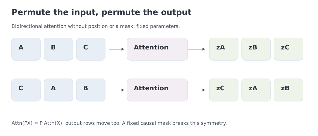 Bidirectional self-attention is permutation-equivariant without a positional signal. A causal mask breaks full symmetry, but it does not by itself provide a rich distance geometry.
2. A map of where position enters
Positional encoding (PE) introduces token coordinates into the computation. RoPE (Rotary Position Embedding) does so by rotating pairs of coordinates.
Position can change the input embedding, the projected query and key, or the score just before softmax. The last quantity is an attention logit: one number controlling a query–key connection. Each approach modifies a different step of the computation from M3.
| Entry point | Operation | Example and section |
|---|---|---|
| Input representation | add a vector indexed by position | sinusoidal PE, §§3–4 |
| Projected query and key | rotate coordinate pairs by position-dependent angles | RoPE, §§4–7 |
| Attention logit | add a distance-dependent bias | ALiBi, §8 |
| No separate positional term | learn order-sensitive behavior from the causal mask and layers | NoPE, §9 |
PI, NTK-aware scaling, and YaRN modify the RoPE frequency spectrum (§7). M-RoPE assigns coordinate pairs to several axes (§13). Treat these names as destinations on the map; you do not need their formulas yet.
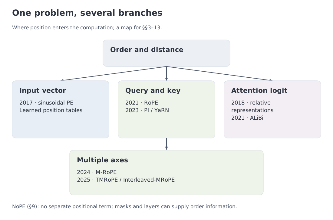 The branches differ in where and how they introduce position. A later method does not replace every earlier one.
Historical connections — optional reading
The original Transformer used deterministic sinusoidal positional encoding. Each position was mapped to a geometric ladder of sine and cosine frequencies. The representation contained no learned positional parameters and could be evaluated beyond the training table.
Learned absolute embeddings offered an even simpler interface: position selected row of a parameter matrix. They work well inside the trained range but tie the architecture to a finite table unless an explicit extension procedure is introduced.
Relative methods moved the positional signal closer to attention. Shaw et al. added learned relative representations. Transformer-XL designed a relative formulation compatible with recurrent segment memory. ALiBi later showed that a head-specific linear distance penalty could provide a surprisingly strong extrapolation prior without rotating or adding embeddings.
RoPE—Rotary Position Embedding—became a particularly influential decoder design. It represents absolute position as a rotation but makes the query-key dot product depend on relative phase. The operation changes neither tensor width nor KV-cache layout.
Long-context work created another branch. Position Interpolation compresses new positions into the old phase range. Community-developed NTK-aware methods change the frequency ladder non-uniformly. YaRN blends original and interpolated frequencies through a ramp. LongRoPE searches dimension-specific extension factors. Llama3-style scaling, partial RoPE, RoPE/NoPE hybrids, local attention, and attention-temperature tuning solve related problems with different assumptions.
Multimodal models then changed the question itself. An image needs height and width. Video adds time. A streaming audio-video model needs time IDs that mean the same thing across modalities. M-RoPE and TMRoPE turn a one-dimensional token index into a small coordinate system.
3. Fourier intuition, complex rotations, and what is exact
Let be an integer position counted from zero. Pair has angular frequency , measured in radians per position step. Its phase is the angle . Frequency tells us how much that angle changes when we advance by one position.
A sinusoidal encoding maps a position to periodic coordinates such as
For the pure positional vectors, the dot product of one sine-cosine pair is exactly relative:
This identity concerns the positional vectors themselves. To understand its effect on attention, we also need to know where they enter the computation. In additive positional encoding, content and position are summed before learned projections. Cross-terms appear, so the final attention score need not be a pure function of .
RoPE rotates the projected queries and keys. Picture each coordinate pair as an arrow in a plane: turning both arrows by the same angle leaves their dot product unchanged.
Optional complex notation. Write the pair as , with now denoting the imaginary unit. Rotation is multiplication by
The common phase cancels in the inner product, leaving a rotation by the relative displacement. This is a direct algebraic property of the query-key geometry.
The Fourier-features analogy remains valuable, but it should not be read too literally. Random Fourier Features sample frequencies to approximate a chosen kernel. Transformer sinusoidal and rotary frequencies are deterministic and geometrically spaced; they are an architectural basis, not a random kernel estimator.
4. Formalism: the frequency ladder and the rotary identity
Here is an even number of rotated coordinates, not the residual width . Full-head RoPE has ; additive PE uses the same frequency construction at the input-vector width. Code often calls these values inv_freq, because they are reciprocals of the phase denominators. A base greater than one controls how quickly frequency falls across pairs.
For an even rotated width , define inverse frequencies
Their wavelengths in token positions are
Classic sinusoidal encoding uses
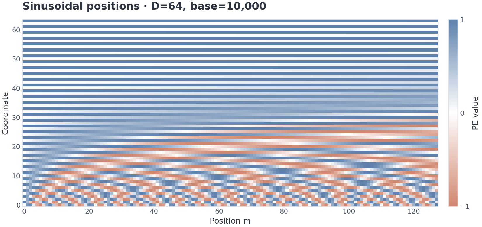 Rows are positional coordinates. Adjacent rows form sine–cosine pairs; higher-index pairs vary more slowly.
RoPE turns the same phase into a rotation matrix:
For a query at position and a key at position ,
and
RoPE therefore uses absolute position IDs to construct rotations, while the positional contribution to the bilinear score enters through the relative displacement . The full score still depends on the content carried by and .
There are two common coordinate layouts. Pedagogical derivations often rotate adjacent pairs , , and so on. Llama-style rotate_half pairs the first half of the vector with the second. They are equivalent under a fixed permutation, not interchangeable on the same trained weights.
The rotation preserves pairwise norms and leaves the tensor shape unchanged. It does not commute with an arbitrary learned matrix. The actual model order is simple: project the residual stream into and , then rotate those projected vectors.
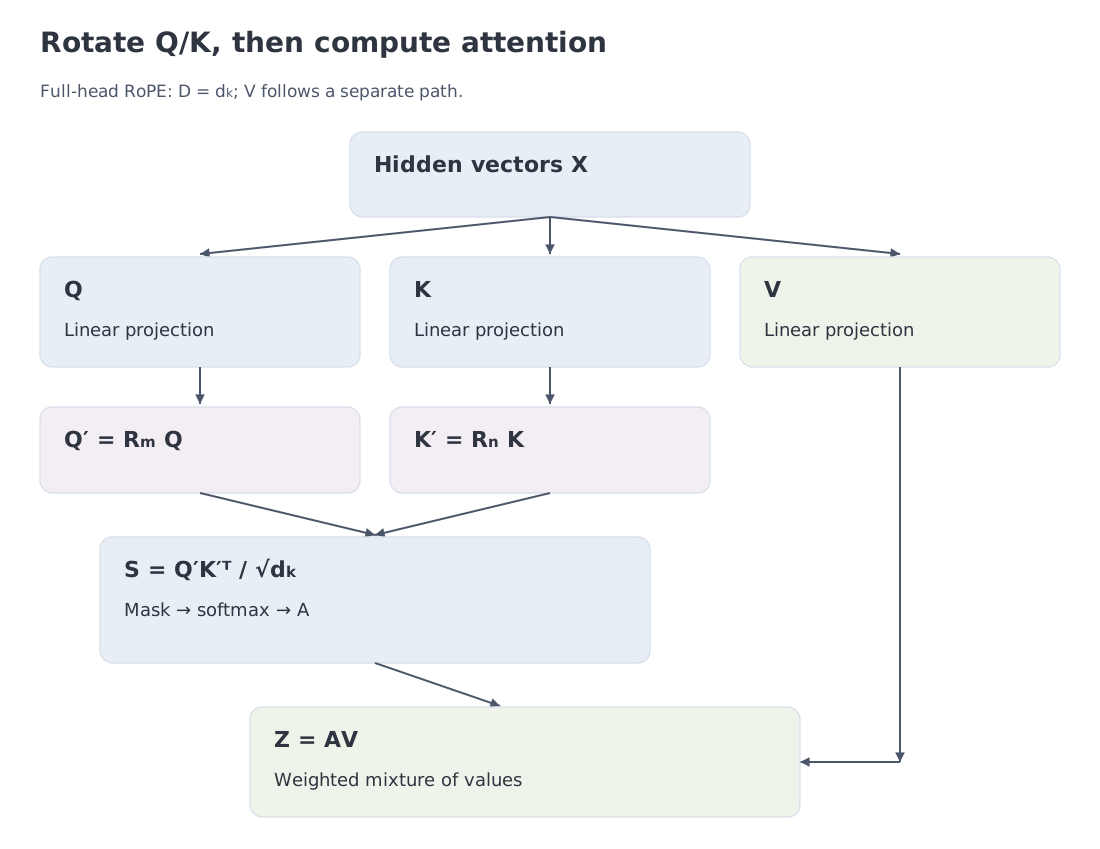 Project to Q/K/V, rotate Q and K, form scaled scores, then mix V. The version shown leaves V unrotated.
Partial RoPE. Some models rotate only D coordinates of a wider head, leaving the remaining channels unchanged. Frequencies use the rotated width D; attention normalization uses the full key width . Scaling just the rotary channels does not multiply the entire dot product by one common factor.
NumPy and PyTorch implementation — second pass
NumPy → PyTorch · B02 — RoPE: rotating coordinate pairs
Implementation route. Assume a validated, nonempty floating tensor x[..., T, D], even D, nonnegative integer IDs [T], and a finite base greater than one. Adjacent coordinates form pairs. The notebook adds input validation (§12).
import numpy as np
import torch
1. Explicit NumPy implementation
def numpy_rope_explicit(
    x: np.ndarray,
    position_ids: np.ndarray,
    *,
    base: float = 10_000.0,
) -> np.ndarray:
    dim = x.shape[-1]
    inv_freq = base ** (-np.arange(0, dim, 2) / dim)
    angles = position_ids[:, None] * inv_freq[None, :]
    shape = (1,) * (x.ndim - 2) + angles.shape
    cos, sin = np.cos(angles).reshape(shape), np.sin(angles).reshape(shape)
    even, odd = x[..., 0::2], x[..., 1::2]
    out = np.empty_like(x, dtype=np.result_type(x.dtype, np.float64))
    out[..., 0::2] = even * cos - odd * sin
    out[..., 1::2] = even * sin + odd * cos
    return out
NumPy exposes inverse frequencies, absolute-position angles, and both coordinates of every 2D rotation, making the positional contribution visible.
2. The same mathematics as explicit PyTorch operations
def torch_rope_explicit(
    x: torch.Tensor,
    position_ids: torch.Tensor,
    *,
    base: float = 10_000.0,
) -> torch.Tensor:
    dim = x.shape[-1]
    work_dtype = torch.float64 if x.dtype == torch.float64 else torch.float32
    inv_freq = base ** (-torch.arange(0, dim, 2, device=x.device, dtype=work_dtype) / dim)
    angles = position_ids.to(device=x.device, dtype=work_dtype)[:, None] * inv_freq[None, :]
    shape = (1,) * (x.ndim - 2) + tuple(angles.shape)
    cos, sin = angles.cos().reshape(shape), angles.sin().reshape(shape)
    even, odd = x[..., 0::2].to(work_dtype), x[..., 1::2].to(work_dtype)
    out = torch.stack((even * cos - odd * sin, even * sin + odd * cos), dim=-1).flatten(-2)
    return out.to(x.dtype)
Phase construction and rotation use at least float32 before conversion back to the input dtype. This avoids early FP16/BF16 position rounding. Float64 remains the reference for large indices: keeping IDs as integers does not remove error after conversion to a working float type. Gradients flow through the input vectors.
| Aspect | NumPy | PyTorch |
|---|---|---|
| Frequencies | np.arange on a CPU array | torch.arange(..., device=x.device) |
| Trigonometry | np.cos, np.sin | Tensor.cos, Tensor.sin |
| Device | CPU | CPU/CUDA/MPS |
| Gradients | none | autograd through the input |
| Precision | float64 calculation and output | float32/64 phases; output keeps input dtype |
| Absolute position | explicit position_ids | must agree with cached-key positions |
Executable parity and edge-case check
rng = np.random.default_rng(2)
x_np = rng.standard_normal((2, 5, 8))
pos_np = np.arange(5, dtype=np.int64) + 11
np_out = numpy_rope_explicit(x_np, pos_np)
x = torch.tensor(x_np, dtype=torch.float64, requires_grad=True)
t_out = torch_rope_explicit(x, torch.tensor(pos_np))
np.testing.assert_allclose(np_out, t_out.detach().numpy(), rtol=1e-12, atol=1e-12)
t_out.square().sum().backward()
# A rotation is orthogonal: d ||R x||^2 / dx = 2 x.
torch.testing.assert_close(x.grad, 2 * x.detach(), rtol=1e-12, atol=1e-12)
# Half-precision IDs would merge 2048 and 2049 before the rotation.
long_ids = torch.tensor([2048, 2049], dtype=torch.int64)
half_x = torch.ones((2, 8), dtype=torch.float16)
half_out = torch_rope_explicit(half_x, long_ids)
expected = numpy_rope_explicit(half_x.numpy(), long_ids.numpy())
np.testing.assert_allclose(half_out.numpy(), expected, rtol=1e-3, atol=1e-3)
assert not torch.equal(half_out[0], half_out[1])
assert long_ids.to(torch.float16)[0] == long_ids.to(torch.float16)[1]
print("B02 outputs, analytic gradient, and float16 positions: PASS")
Complete executable file: m04_rope_bridges.py
5. Worked example: three placements, one relative displacement
Let
with head dimension four and base 10,000. The inverse frequencies are
Place the query at position 3 and the key at position 1. Using adjacent coordinate pairs, their rotated dot product before attention scaling is
Now shift both tokens by four positions. The pair has the same displacement as , so the result is unchanged. The pair gives the same value as well.
| query position | key position | unscaled dot product | |
|---|---|---|---|
| 3 | 1 | 2 | 1.144248 |
| 7 | 5 | 2 | 1.144248 |
| 2 | 0 | 2 | 1.144248 |
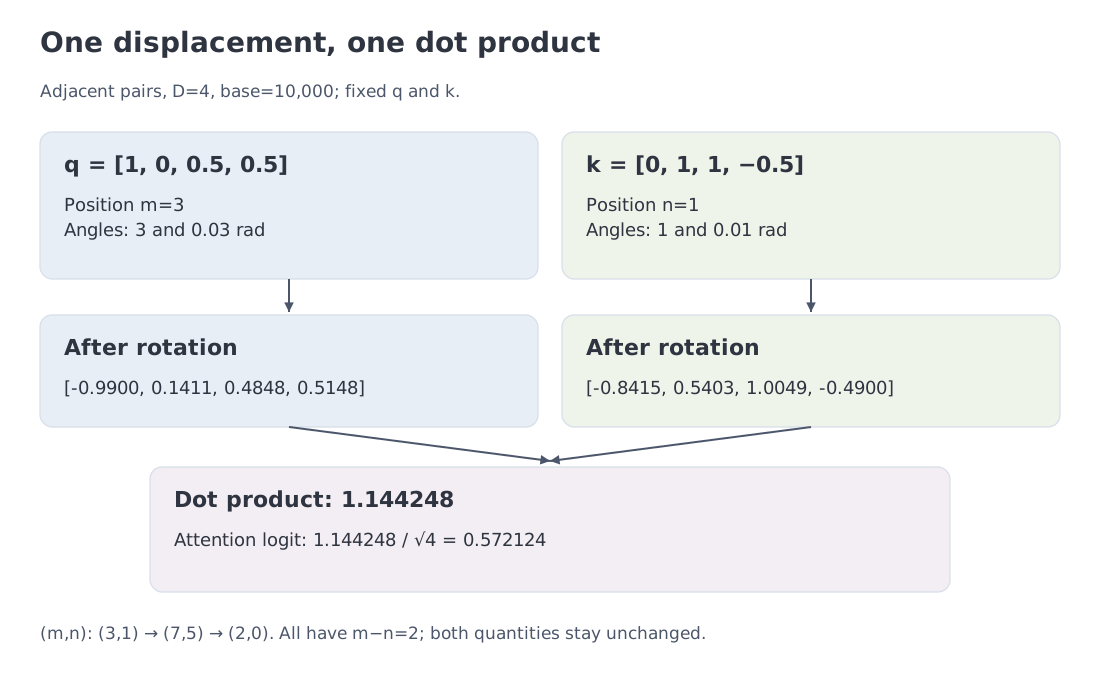 Absolute angles change across placements, but a shared relative displacement preserves the same unscaled dot product.
To obtain the standard attention logit from M3, divide by , giving approximately 0.572124. Masking and softmax follow. This constant scaling preserves the common-shift identity.
The identity is exact for fixed and . In a network, those vectors still depend on content and layer state, so attention does not reduce to a distance-only kernel.
6. Reading the RoPE frequency spectrum
The base parameter controls a geometric spectrum. The fastest pair is always
regardless of base. Increasing rope_theta therefore does not remove the fastest local phase. It mainly slows the higher-index pairs, allocating more of the spectrum to long wavelengths.
The diagnostic is : turns across a span of L position steps, following the YaRN convention. A sequence indexed from 0 to L−1 has endpoint separation L−1. These are different quantities. Wavelengths below are measured in position steps.
For :
| base | minimum wavelength | maximum wavelength | pairs with ≥1 turn by 4096 |
|---|---|---|---|
| 10,000 | 6.28 | 47,117 | 23 of 32 |
| 150,000 | 6.28 | 649,409 | 18 of 32 |
| 500,000 | 6.28 | 2,084,765 | 16 of 32 |
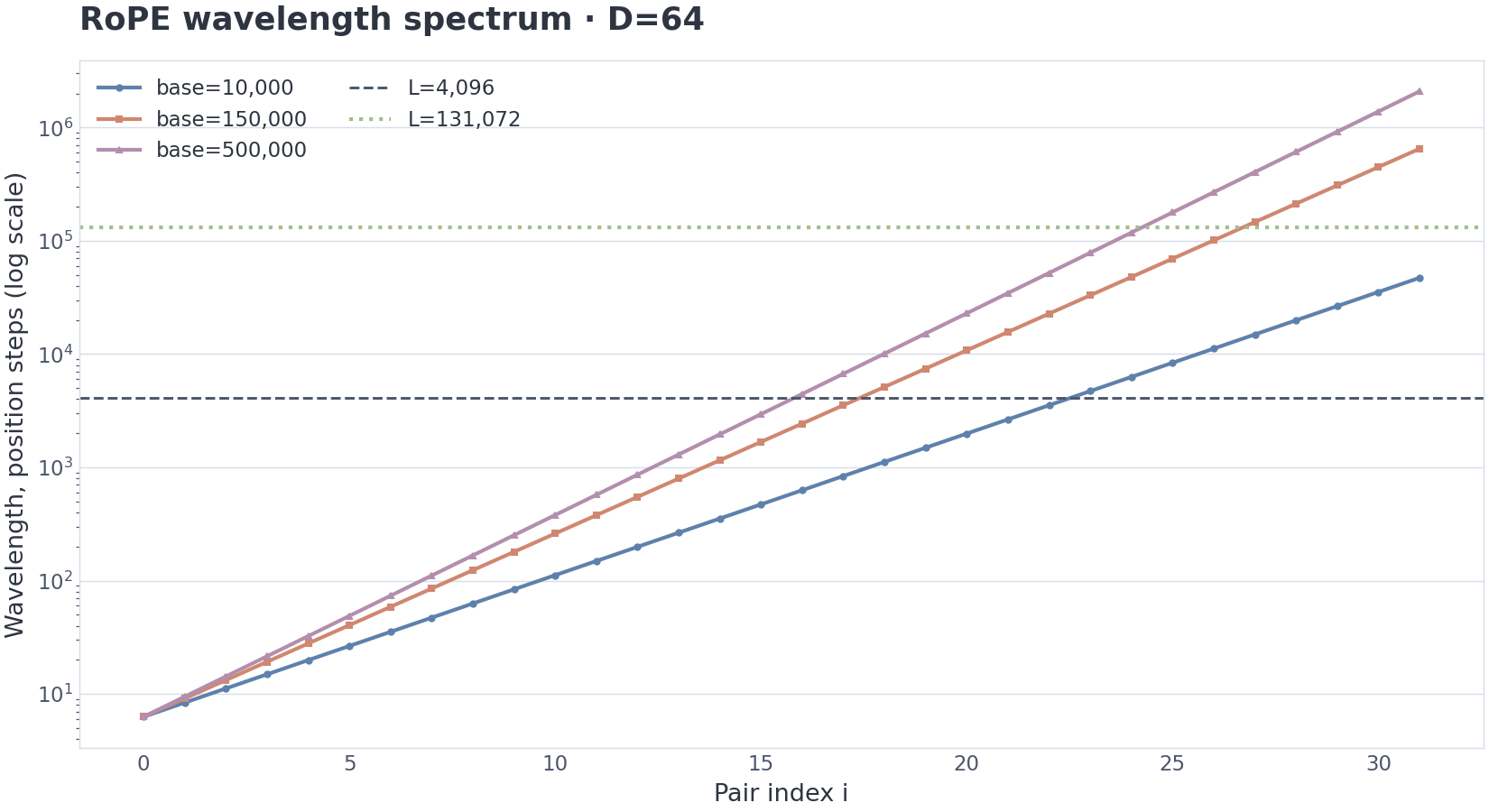 Wavelengths show how a base redistributes phases. Context-length guide lines are diagnostics, not a global period for the full positional vector.
Each coordinate pair is periodic. The complete representation combines many different periods. One pair returning to a similar angle does not make two full positional vectors identical. Consequently, the largest wavelength of one pair is not a hard context limit, and a small base does not imply that every position beyond that wavelength becomes indistinguishable.
Turn counts still convey useful information. Fast pairs sweep through many phases during training; slow pairs may cover only a small arc. Extrapolating those slow coordinates sends the model into new phase regions. That is an out-of-distribution geometry, not a mathematical prohibition. Whether the model uses it successfully is empirical.
7. Context extension changes a spectrum, not just one number
Let be the reference length used to set the frequencies, and let be an extension factor. We want to process tokens. In a research experiment, is often the training length; a configuration field alone does not establish the full training history (§10).
Position Interpolation
Position Interpolation maps to . Equivalently,
The new range stays inside familiar angular values. The cost is that all local phases are compressed as well. Fine-tuning is normally used to help the model adapt to this altered geometry.
Static NTK-aware scaling
A widely used static heuristic changes the base to
This leaves the fastest end of the spectrum less changed and slows the low-frequency end more aggressively. “NTK-aware” describes the motivation, not a general theorem guaranteeing safe zero-shot extension.
Assume and . Substituting the new base gives : pair zero is unchanged, while the final pair slows by exactly s. The expression is undefined at D=2. NTK stands for Neural Tangent Kernel, a theoretical description of wide networks; this calculation uses only the stated base-change rule.
YaRN
YaRN builds an original spectrum and a fully interpolated spectrum, then blends them through a frequency-dependent ramp. A diagnostic number of rotations within the reference context determines the ramp boundaries.
Define , the number of turns over the reference span. Two thresholds, , select the transition: fast pairs keep their original frequencies, while slow pairs use interpolation. Solving gives a fractional pair index:
A ramp is a linear transition clipped to the interval [0,1]:
Zero selects the original frequency; one selects full interpolation. Intermediate weights blend the two. Our example has distinct boundaries inside the spectrum; the teaching implementation rejects a collapsed range.
For the module scenario
head_dim = 64
base = 150000
reference length = 4096
factor = 32
beta_fast = 32
beta_slow = 1
the original gpt-oss implementation uses the continuous bounds
Those values still divide the integer-indexed pairs into three groups:
- 9 pairs remain at their original frequencies;
- 9 pairs occupy the transition ramp;
- 14 pairs are fully interpolated.
The generic Hugging Face YaRN utility also offers truncate=True, which rounds the boundaries to low=8, high=18. GptOssConfig sets truncate=False, so the continuous values are the faithful default for this model.
In this particular configuration, the fully interpolated set coincides with pairs that complete less than one turn in the reference context. That is a property of the chosen boundary formula and hyperparameters, not a universal rule that one full turn makes extrapolation “safe.”
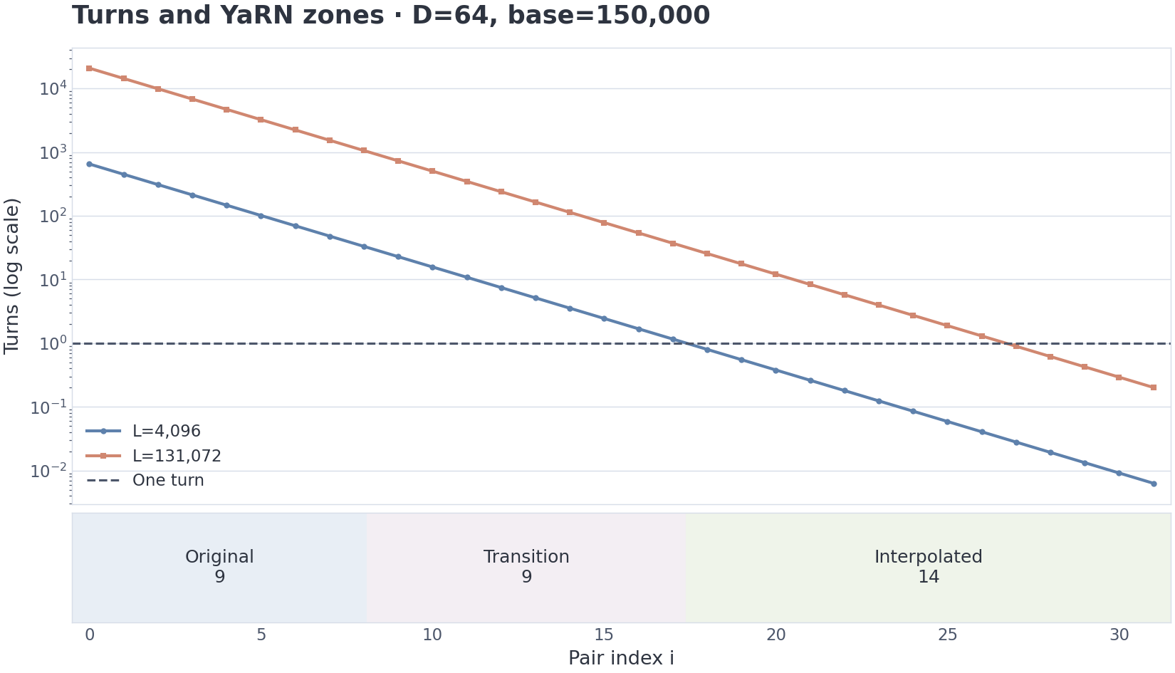 Turn counts help define the teaching YaRN ramp. The zones mean original, transition, and interpolated—not mathematically allowed and forbidden.
YaRN also adjusts attention concentration. Temperature divides logits before softmax; lowering it makes a fixed set of scores more uneven. An attention_factor can implement this by scaling the rotated vectors. The original gpt-oss implementation and its Hugging Face adaptation use this approach. For , both checked paths use
At , . Both checked implementations apply this factor to computed rotary cosines and sines. If both rotated queries and keys therefore receive the same factor, their dot product is scaled by
The whole-score factor assumes that every query and key coordinate receives a. With partial RoPE, only the rotary contribution is scaled unless the remaining channels are adjusted separately. The fitted rule for a is empirical, not a consequence of rotation algebra.
Another runtime may move the equivalent scaling into queries, keys, or the attention score. A configuration field only becomes unambiguous when read with the implementation that consumes it.
Beyond one scaling recipe
LongRoPE searches per-dimension factors and can use different regimes for different lengths. LongRoPE2 incorporates training-aware criteria. Llama3-style scaling divides the spectrum into wavelength bands. Other models use partial RoPE, interleaved RoPE/NoPE, local attention, or length-dependent attention temperature.
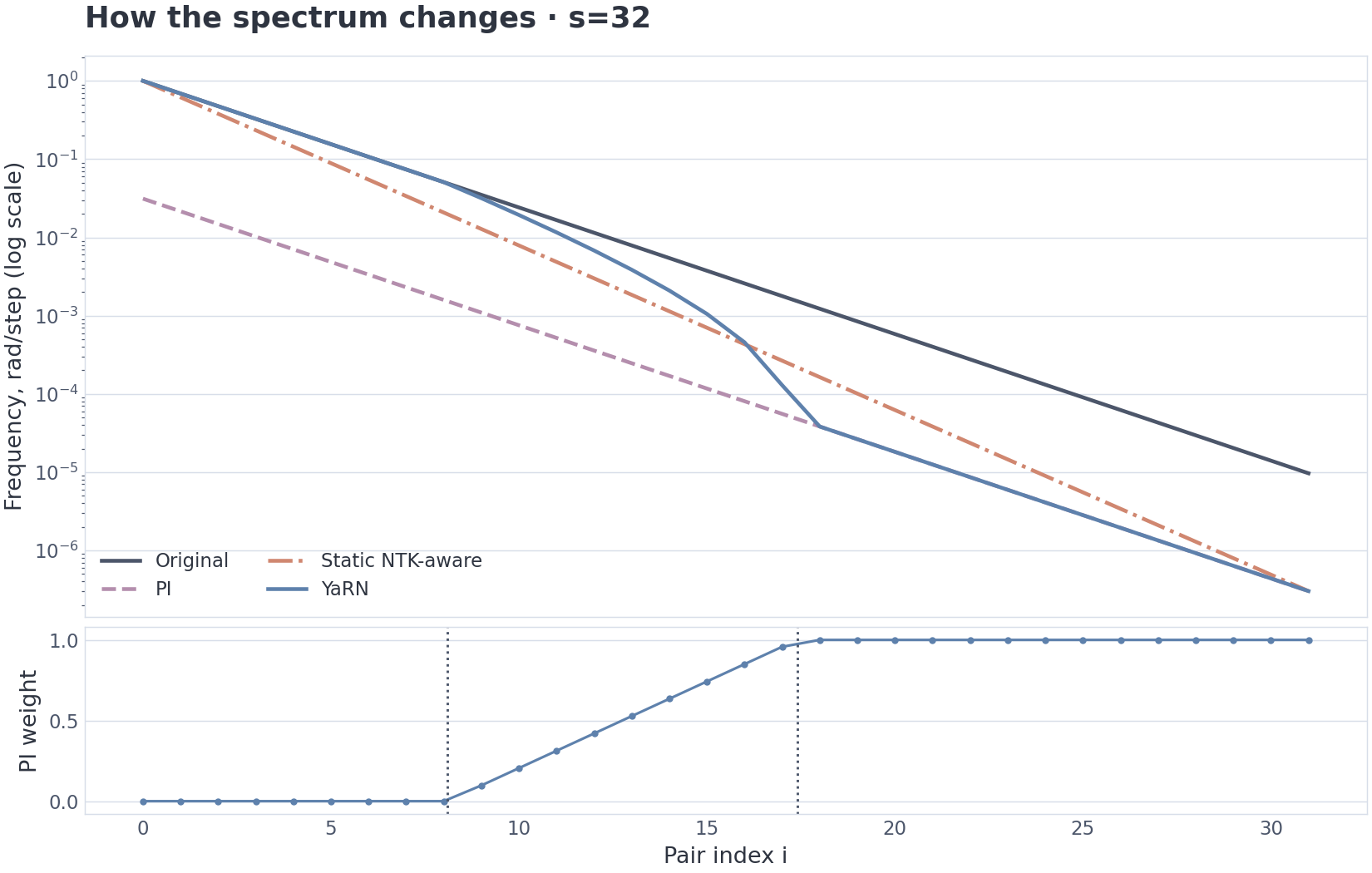 PI, static NTK-aware scaling, and YaRN reshape the same starting spectrum differently. The figure compares geometry, not guaranteed downstream quality.
8. ALiBi: a distance prior in the logits
ALiBi—Attention with Linear Biases—leaves queries and keys untouched. Head receives a slope , and causal attention uses
The slope is fixed per head and measured in logit units per position step. A separate causal mask excludes future keys; a finite ALiBi penalty cannot replace it.
Heads with steeper slopes favor nearby context more strongly. If the content score were fixed, softmax would turn the linear penalty into an exponential distance prior:
The complete attention pattern is not a stationary kernel by itself; it still depends on content and normalization across available keys.
ALiBi's strength is structural simplicity and a bias that continues to any distance. Its limitation is equally clear: the form of the distance prior is fixed in advance.
One common measure of next-token prediction is perplexity, , using M3's mean negative log-likelihood in nats per evaluated token. On the same data, with the same tokenizer and evaluation mask, lower perplexity means that the model assigns higher probability, on average, to the observed continuations. Maintaining this score at longer lengths does not establish reliable retrieval from the middle of a document or reasoning across distant evidence. Those require separate evaluations.
9. NoPE and hybrid position mechanisms
NoPE—No Positional Encoding—removes an explicit positional term. A causal model is not deprived of all order information: the mask, depth, and recursively constructed hidden states expose asymmetries tied to prefix length.
Research shows that substantial positional behavior can emerge under these conditions. That does not make explicit position universally unnecessary. It means the model can infer part of the structure from other components of the computation.
Two cases should be separated:
- pure NoPE, where no layer receives an explicit positional encoding;
- hybrid designs, where some layers use RoPE and others NoPE, or where positional mechanisms are combined with different attention patterns.
Llama 4 is a concrete hybrid. Its open configuration supports a NoPE layer at a regular interval, chunked attention, and length-dependent temperature tuning. In the Llama 4 implementation, enabling attn_temperature_tuning scales queries in NoPE layers. This is separate from the YaRN frequency ramp.
10. Reading the gpt-oss positional configuration
This example uses the original gpt-oss-120b configuration at revision b5c939de…. The module includes its bytes and checksum, so later edits to main cannot change the exercise. We checked it against OpenAI revision 7b583341… and Transformers revision 536ecc007… on 10 October 2026.
The relevant fields are
{
  "head_dim": 64,
  "initial_context_length": 4096,
  "rope_theta": 150000,
  "rope_scaling_factor": 32.0,
  "rope_ntk_alpha": 1,
  "rope_ntk_beta": 32
}
This is enough to reconstruct a positional geometry:
- 32 rotary pairs per head;
- base 150,000;
- a reference length of 4,096;
- a 32-fold extension factor;
- correction-boundary parameters corresponding to 1 and 32 rotations.
The module's transparent reconstruction therefore gives the continuous bounds low≈8.0928, high≈17.3980, together with the default attention factor 1.346574. The integer pair 8/18 belongs to the optional truncate=True mode, not to the original gpt-oss path.
What the file does not provide is a complete training chronology. initial_context_length tells us the reference length used by the scaling contract. It does not, by itself, prove that all pretraining happened at 4K and that one particular extension phase followed. Such claims require a technical report or training recipe.
Converted Hugging Face configurations may express the same information through a more general RoPE parameter dictionary. Field names and scaling placement can change across representations, so the config should be read together with the model code and library revision.
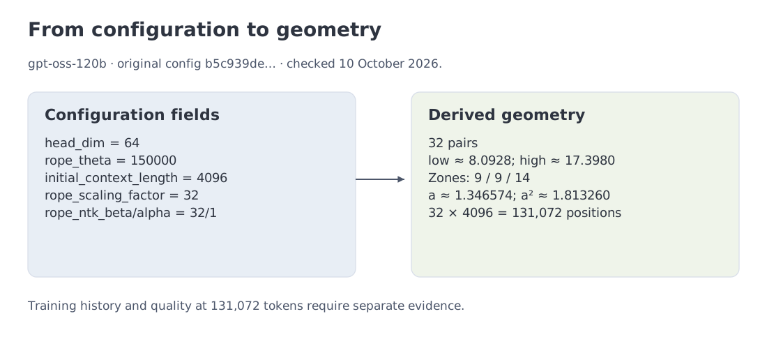 The gpt-oss fields support a reconstruction of the positional spectrum. They do not constitute a complete training schedule.
11. Level-one code: explicit shapes and explicit scaling placement
The following NumPy code is designed for inspection rather than fused execution. It validates head width, positions, frequency shape, and the YaRN ramp. The pairing convention is the split-half rotate_half layout used by Llama-like implementations.
The compact apply_rope below requires equal Q/K shapes and one shared position vector. It represents a full sequence block; the notebook rotates queries and cached keys separately when their lengths differ. This core calculates in float64 and returns the YaRN amplitude for the caller to apply. It covers the declared scenario, not every library variant.
import math
import numpy as np

def rope_inv_freq(head_dim: int, base: float = 150_000.0) -> np.ndarray:
    """Return theta_i = base**(-2i/D) for D/2 rotary pairs."""
    if isinstance(head_dim, bool) or not isinstance(head_dim, int):
        raise TypeError("head_dim must be an integer")
    if head_dim < 2 or head_dim % 2:
        raise ValueError("head_dim must be positive and even")
    if not math.isfinite(base) or base <= 1.0:
        raise ValueError("base must be finite and greater than 1")
    i = np.arange(head_dim // 2, dtype=np.float64)
    return base ** (-2.0 * i / head_dim)

def rotate_half(x: np.ndarray) -> np.ndarray:
    """Quarter-turn the split-half coordinate pairs."""
    if x.ndim < 2 or x.size == 0 or x.shape[-1] % 2:
        raise ValueError("x must have shape [..., T, D] with even D")
    half = x.shape[-1] // 2
    return np.concatenate((-x[..., half:], x[..., :half]), axis=-1)

def apply_rope(q, k, positions, inv_freq):
    """Apply split-half RoPE to q/k of shape [..., T, D]."""
    if any(np.iscomplexobj(x) for x in (q, k, inv_freq)):
        raise TypeError("q, k and inv_freq must be real")
    q = np.asarray(q, dtype=np.float64)
    k = np.asarray(k, dtype=np.float64)
    positions = np.asarray(positions)
    inv = np.asarray(inv_freq, dtype=np.float64)
    if q.shape != k.shape or q.ndim < 2 or q.size == 0 or q.shape[-1] % 2:
        raise ValueError("q and k must share shape [..., T, D], with even D")
    if not np.isfinite(q).all() or not np.isfinite(k).all():
        raise ValueError("q and k must be finite")
    if positions.ndim != 1 or positions.dtype.kind not in "iu":
        raise ValueError("positions must be an integer vector [T]")
    if positions.size != q.shape[-2] or np.any(positions < 0):
        raise ValueError("positions do not match the sequence axis")
    if inv.shape != (q.shape[-1] // 2,) or not np.isfinite(inv).all() or np.any(inv <= 0):
        raise ValueError("inv_freq must be positive and have shape [D/2]")

    angles = positions.astype(np.float64)[:, None] * inv[None, :]
    angles = angles.reshape((1,) * (q.ndim - 2) + angles.shape)
    if not np.isfinite(angles).all():
        raise FloatingPointError("phase overflow")
    full = np.concatenate((angles, angles), axis=-1)
    cos, sin = np.cos(full), np.sin(full)
    qr, kr = q * cos + rotate_half(q) * sin, k * cos + rotate_half(k) * sin
    if not np.isfinite(qr).all() or not np.isfinite(kr).all():
        raise FloatingPointError("rotation overflow")
    return qr, kr

def yarn_inv_freq(head_dim, base, factor, original_context,
                  beta_fast=32.0, beta_slow=1.0, *, truncate=False):
    """Blend original and interpolated frequencies with a YaRN-style ramp."""
    inv = rope_inv_freq(head_dim, base)
    if not math.isfinite(factor) or factor < 1.0:
        raise ValueError("factor must be at least 1")
    if isinstance(original_context, bool) or not isinstance(original_context, int):
        raise TypeError("original_context must be an integer")
    if not math.isfinite(beta_fast) or not math.isfinite(beta_slow):
        raise ValueError("beta parameters must be finite")
    if original_context <= 0 or beta_fast <= beta_slow or beta_slow <= 0:
        raise ValueError("invalid context or beta parameters")
    if not isinstance(truncate, bool):
        raise TypeError("truncate must be bool")

    def correction_dim(turns: float) -> float:
        return head_dim * math.log(
            original_context / (turns * 2 * math.pi)
        ) / (2 * math.log(base))

    pair_count = head_dim // 2
    low_raw = correction_dim(beta_fast)
    high_raw = correction_dim(beta_slow)
    low = math.floor(low_raw) if truncate else low_raw
    high = math.ceil(high_raw) if truncate else high_raw
    low = min(max(float(low), 0.0), float(pair_count - 1))
    high = min(max(float(high), 0.0), float(pair_count - 1))
    if high <= low:
        raise ValueError("the YaRN ramp collapsed")

    ramp = np.clip(
        (np.arange(pair_count, dtype=np.float64) - low) / (high - low),
        0.0,
        1.0,
    )
    scaled = inv * (1.0 - ramp) + (inv / factor) * ramp
    attention_factor = 1.0 if factor <= 1 else 1.0 + 0.1 * math.log(factor)
    return scaled, attention_factor, attention_factor**2, low, high
The last function returns both the rotary factor and the score factor implied when the same scaling enters queries and keys. Keeping them separate prevents a common ambiguity in configuration discussions.
13. M-RoPE and time-aligned multimodal position
M-RoPE—Multimodal Rotary Position Embedding—assigns different sections of rotary channels to temporal, height, and width coordinates. A single attention operation can therefore represent text and visual geometry without switching to a separate positional mechanism.
Text uses the same ID on all three axes:
Every frequency pair therefore receives the ordinary one-dimensional position , regardless of which section it belongs to. The text path is equivalent to standard 1D RoPE.
A still image holds temporal position constant and varies its two spatial coordinates:
A grid can be represented as
Video changes all three axes. Qwen2.5-VL can space temporal IDs according to real time between grid elements rather than treating frame number as the only clock.
TMRoPE—Time-aligned Multimodal Rotary Position Embedding—was documented in the Qwen2.5-Omni technical report in March 2025. It aligns audio and video timestamps. In that model, one temporal ID corresponds to 40 ms. This is a model-specific time grid, not a universal definition of TMRoPE.
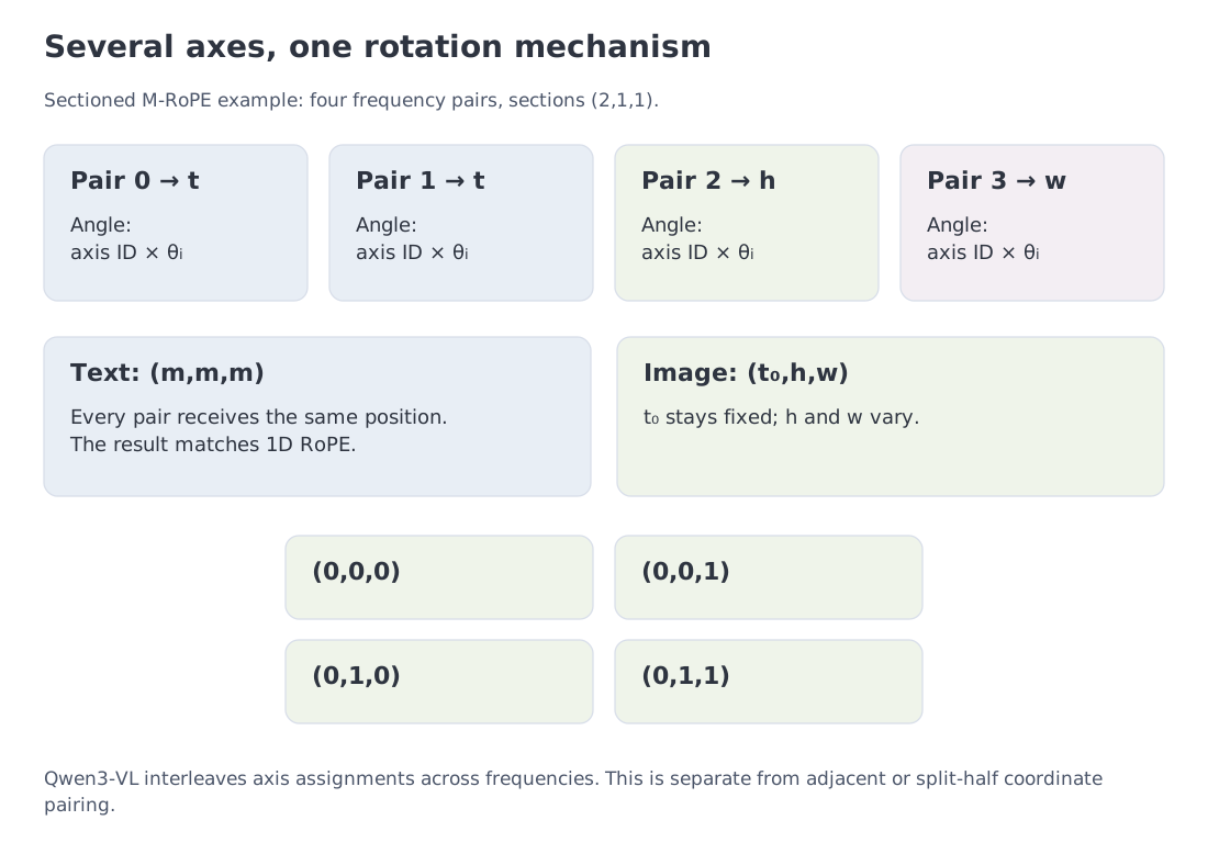 Text repeats one position ID across all axes; images vary height and width at fixed time; video and synchronized audio use a temporal coordinate.
Interleaved axes in Qwen3-VL
Sectioned M-RoPE gives time, height, and width separate frequency groups. Qwen3-VL, §2.1 instead interleaves axis assignments across frequency pairs, giving each axis access to faster and slower bands. This is Interleaved-MRoPE. Axis allocation is separate from the adjacent-versus-split-half layout of the two coordinates inside each pair.
The report also describes explicit textual video timestamps (§2.3). The 40 ms grid from Qwen2.5-Omni is therefore not a family-wide rule. Our 2×2 example implements sectioned M-RoPE, not a complete Qwen3-VL position system. Mixed text and visual sequences also need a convention for coordinate offsets and the text that follows; the toy grid starts at zero for clarity.
14. The 2026 landscape is a branching architecture map
This selective implementation map was checked on 10 October 2026. Use it as a reference after learning the mechanisms: each row points to evidence for a particular positional design, not a ranking or an exhaustive catalogue.
| Family or method | Positional mechanism | Purpose or context | Evidence |
|---|---|---|---|
| Transformer | deterministic sinusoidal PE | original sequence architecture | paper |
| RoFormer / RoPE | rotation in | relative phase in attention | paper |
| ALiBi | linear logit bias | length extrapolation without a position table | paper |
| Position Interpolation | uniform position compression plus tuning | RoPE context extension | paper |
| YaRN | original/interpolated spectral ramp plus scaling | long-context extension | paper and runtime implementations |
| LongRoPE / LongRoPE2 | per-dimension and length-dependent factors | very long context | papers |
| gpt-oss | base 150K, reference length 4096, factor 32, correction parameters | up to 128K positional configuration | official config; config alone is not a training schedule |
| Llama 4 | interleaved RoPE/NoPE, chunked attention, temperature tuning | hybrid long-context stack | open configuration and implementation |
| Qwen2-VL / Qwen2.5-VL | M-RoPE | text, image, and video coordinates | paper and code |
| Qwen2.5-Omni | TMRoPE | aligned audio-video time | technical report |
| Qwen3-VL | Interleaved-MRoPE and textual timestamps | frequency allocation across axes and video event timing | report, §2 and open implementation |
| Inkling | relative positional embeddings with sliding/global layers | 1M context | official architecture announcement |
| Closed API models | may be undisclosed | advertised window does not reveal the formula | provider documentation only where available |
A context-window number does not identify the positional mechanism, and it does not establish reliable use of every position inside the window. Operational context quality is an evaluation problem, addressed later in Module 19.
17. Key takeaways
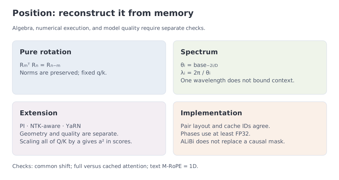 Permutation symmetry, rotary relativity, spectral diagnostics, context-scaling families, ALiBi/NoPE, and multimodal axes on one page.
- Bidirectional self-attention without position is permutation-equivariant. A causal mask supplies access order, not a complete distance geometry.
- Pure sinusoidal pairs already have an exact relative dot product. RoPE inserts relative phase directly into the projected query-key score.
rope_thetaredistributes a frequency ladder. A larger base introduces slower components without removing the fastest pair.- A single wavelength or turn count is not a hard context boundary.
- PI compresses every frequency; static NTK-aware scaling is a heuristic; YaRN blends original and interpolated spectra; other long-context families make different trade-offs.
attention_factormust be interpreted at the point where the runtime applies it.- ALiBi is a linear positional bias. NoPE can be pure or part of a hybrid stack.
- M-RoPE repeats IDs for text and uses multiple axes for visual tokens. TMRoPE aligns multimodal time.
- A configuration describes architectural geometry; it is not a substitute for a training report.
Next: Module 5, attention mechanisms. With position accounted for, we can examine how heads are organized and how attention is computed without unnecessary memory use.
18. primary sources
Primary sources:
- Vaswani et al., Attention Is All You Need — arxiv.org/abs/1706.03762
- Shaw et al., Self-Attention with Relative Position Representations — arxiv.org/abs/1803.02155
- Dai et al., Transformer-XL — arxiv.org/abs/1901.02860
- Su et al., RoFormer / RoPE — arxiv.org/abs/2104.09864
- Press et al., ALiBi — arxiv.org/abs/2108.12409
- Haviv et al., positional behavior without explicit PE — arxiv.org/abs/2203.16634
- Chen et al., Position Interpolation — arxiv.org/abs/2306.15595
- Peng et al., YaRN — arxiv.org/abs/2309.00071
- Ding et al., LongRoPE — arxiv.org/abs/2402.13753
- Shang et al., LongRoPE2 — arxiv.org/abs/2502.20082
- Bai et al., Qwen2-VL — arxiv.org/abs/2409.12191
- Xu et al., Qwen2.5-Omni — arxiv.org/abs/2503.20215
- Hugging Face RoPE utilities
- gpt-oss original configuration
- gpt-oss reference RoPE implementation
- Hugging Face GptOssConfig
- Llama 4 model documentation
- Qwen3-VL — report, §2; implementation
- Inkling architecture announcement
Further study. Fourier features, kernels, and information geometry are developed in Information Theory for ML. Recurrent and state-space alternatives to explicit positional encoding appear in later Modern LLMs modules.
Selected implementations checked: 10 October 2026. Spectrum and YaRN numbers belong to an explicitly stated teaching scenario. For closed models, an undisclosed positional mechanism is not inferred from the advertised context window.