Module 11. Speculative Decoding and Quantization
Modern LLMs · Module 11 lecture · revision October 11, 2026
What this module is about. Module 10 ended with an uncomfortable systems fact: during autoregressive decode, a GPU may spend more time moving model state than performing arithmetic. This module studies two ways to change that cost structure. Quantization makes each target-model step move fewer bytes. Speculative decoding tries to make one expensive target step validate several tokens. Both techniques are mature enough to appear in production engines, yet neither comes with a workload-independent speedup. We will keep the mathematics exact where it can be exact, and label every performance number according to what it actually is: a derived scenario, a paper result, or a measured deployment property.
Prerequisites. The distinction between prefill and decode from Module 10 is useful, as is the multi-token prediction objective introduced in Module 9. The necessary definitions are restated here, so the lecture can be read on its own.
Reading routes. On a first pass, follow Sections 1, 3–12, and 15–20. Understand why proposals can preserve a distribution and why fewer stored bits do not imply a fixed speedup. Read the probability table and balance proof in Section 5; extended NumPy/PyTorch blocks can wait.
On a second pass, work through Sections 13–14 and the bridges in Sections 5 and 13, then run the notebook and solve the exercises before opening the answers. The project demos extend local calculations to history-dependent generation and a layer-level quantization experiment.
For reference, Section 2 provides historical context, Sections 8–9 locate proposer families, Sections 11–12 describe representations, and Section 17 records a reproducible run. This route assumes the sampling argument in Sections 4–5.
1. Two different ways to make a token cheaper
During prefill, the model processes known prompt tokens and constructs the keys and values retained in the KV cache. During decode, it extends that prefix. Ordinary autoregressive generation feeds each selected token into the next step. Dependence between steps and the cost of each step are separate problems; this module changes their economics without assuming either disappears.
Consider a model that has already processed its prompt. The KV cache is resident, and the server now needs one more token. In a common low-concurrency regime, the limiting resource is not peak FLOP/s but memory bandwidth: a large amount of model state is read for a comparatively small amount of useful work.
A deliberately narrow model of the weight-streaming limit is
Here is tokens per second for one sequence, is bytes per second, and is bytes read per step. The dense 8B example assumes one read of all weights per step. KV traffic, temporary storage, communication, scheduling, and imperfect utilization are absent. The expression is not a service benchmark; it is a lens for seeing two independent interventions.
Quantization attacks . If an 8B model occupies 16 decimal GB in bf16, a 3.35 TB/s memory system has an arithmetic weight-only limit of 209.4 tokens/s. Eight-bit weights halve the payload. A 4.5-bit-per-weight accounting reduces it to 4.5 GB and raises that particular ceiling to 744.4 tokens/s.
Speculation changes what one target read produces. A cheaper proposer drafts future tokens; the target evaluates several positions in one forward pass. Accepted proposals let a single target invocation advance the sequence by more than one token.
The two methods can be combined because they operate on different parts of the cost. They should not, however, be treated as independent coupons. Once weight traffic falls, another bottleneck may take over; once verification becomes wider, arithmetic and scheduling costs may stop being negligible.
2. From exact sampling to deployable systems
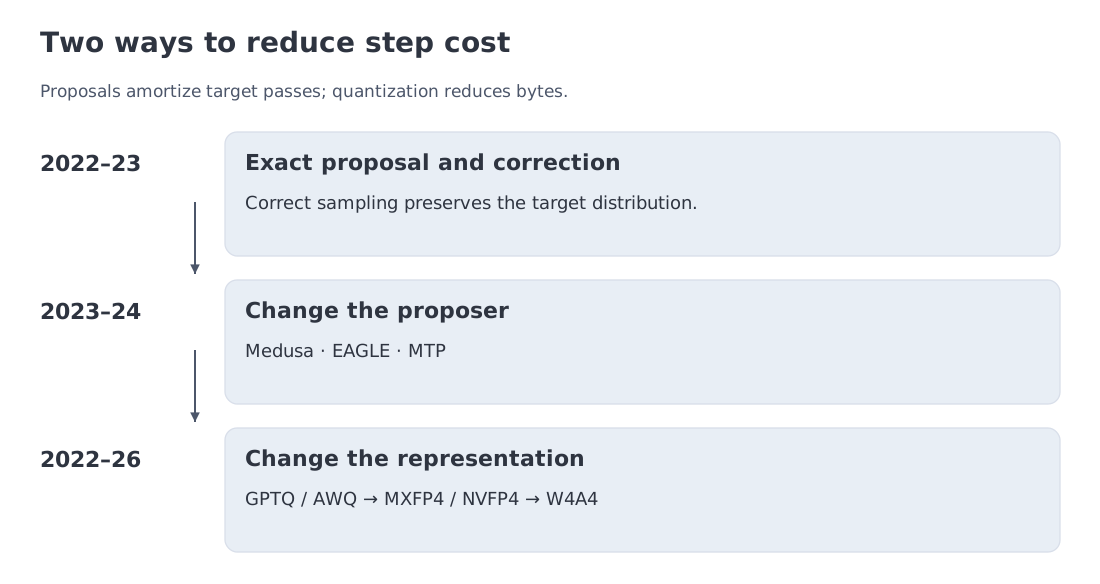 The speculative-decoding line moves from exact rejection-based algorithms to trainable and native proposers. The quantization line moves from INT4 PTQ to microscaled FP4 and hardware-backed W4A4 execution.
The key conceptual step in speculative decoding was not merely “use a small model first.” It was showing how to do so without changing the target distribution. Leviathan, Kalman, and Matias, and independently related work by Chen and colleagues, turned a draft model into a proposal distribution and used a correction step to preserve exact sampling.
Later work focused on the proposer. Medusa attached multiple prediction heads to the target and verified a tree of candidates. EAGLE learned a compact proposer from target-model features; EAGLE-3 moved to direct token prediction and multi-layer feature fusion. Pattern-based approaches took a different route: n-gram, prompt-lookup, and suffix methods propose text that has already appeared in the context or a cache.
Multi-token prediction created a native path. A model trained to predict beyond the next token may retain modules that can serve as internal proposers. The DeepSeek-V3 report explicitly notes speculative decoding as a use of its MTP objective, and current inference engines expose MTP for compatible architectures.
Quantization followed its own progression. GPTQ and AWQ made low-bit post-training quantization practical for LLMs. Methods such as SmoothQuant and rotation-based transforms addressed activation outliers and channel imbalance. FP4 then shifted the problem from “four bits” to which four-bit value grid, which scale hierarchy, and which kernel.
As of October 11, 2026, both topics are better understood as design spaces than as single features. A useful deployment decision must name the proposer, verifier, sampling rule, quantization format, scale granularity, hardware path, and workload.
3. The older ideas underneath the modern stack
Three classical connections make the rest of the module easier to reason about.
The first is rejection sampling. A tractable proposal helps sample from a target . A proposal is accepted according to a likelihood ratio, and rejected mass must be corrected. Speculative sampling adapts this idea to autoregressive models and arranges the correction so that a cycle always makes progress.
The second is speculative execution in processors. Work is performed before it is known to be useful; correct predictions are committed, and incorrect ones are discarded. The LLM analogue is structurally similar, but it carries an additional statistical obligation: the accepted-and-corrected result must have the same distribution as target-only sampling.
The third is block floating point. A short numerical code cannot represent both fine local detail and a large global range unless some range information is shared. Microscaling stores a low-bit value per element and a scale per small block. Smaller blocks track local variation more closely but consume more metadata.
These connections also warn against superficial comparisons. A proposer is not useful because it is small; it is useful when it is cheap and overlaps strongly with the target. A four-bit checkpoint is not fast because its file is small; it is fast only when the runtime can execute the corresponding representation efficiently.
4. The exact propose–verify–correct cycle
The target is the model whose sampling law must be preserved. The draft, or proposer, supplies candidates. At position , both and are conditioned on the same history, including earlier proposals in that cycle. Subscripts are omitted in short equations; probabilities may still change across positions.
Module 3, Section 12.1, worked through temperature → top-k → top-p numerically. Here we use the resulting distributions from which tokens are actually sampled. Temperature changes logit sharpness; top-p retains a smallest set of the most probable tokens reaching a chosen cumulative mass; a grammar mask removes forbidden continuations. With these transformations enabled, describes the transformed proposal law and the transformed target law. Using raw probabilities while sampling from a filtered law breaks the proof.
Let be the target distribution for the next token and the draft distribution over the same token space. The proposer generates autoregressively. The target then evaluates all proposed positions in a batched forward pass.
At position , the proposed token is accepted with probability
Verification proceeds from left to right. At the first rejection, the remaining draft suffix is invalidated and a replacement token is sampled from
The target pass remains causal: the row predicting cannot see later proposals. Aligning inputs and outputs matters because logits at an input position predict the following token. If all proposals survive, the next-position distribution supplies a bonus token. Otherwise, the unaccepted suffix and its cache entries are discarded before continuing from the corrected prefix.
The notation means entry by entry, and divides by the sum. A positive residual exists whenever rejection is possible. End-of-sequence and output-length limits can terminate a cycle early; the progress formula below first considers a cycle without those stopping events.
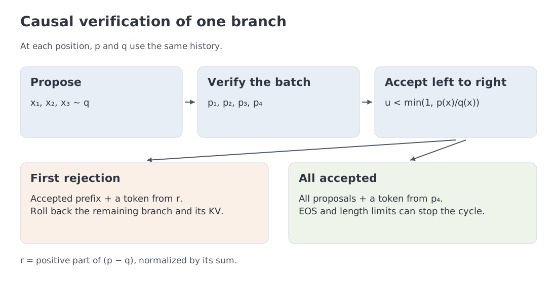 A draft continuation, one batched target verification, left-to-right acceptance, and residual resampling at the first rejection.
The proof fits in a mass-balance identity. Define
The accepted branch emits token with mass . The correction branch is entered with probability and contributes . Therefore
The proposer supplies shared mass; correction supplies the missing target mass. Applying this identity at each reached history preserves the autoregressive law of the full continuation. Distributional equality does not require the same output string under the same seed: the algorithms consume random numbers differently.
This statement is exact under the assumptions of the algorithm. The target and proposer need a compatible token space, the verifier needs target probabilities, and the acceptance/correction rule must be implemented faithfully. A grammar mask fits this proof when it is included in the normalized laws and at the same history. Greedy tree verification, lossy acceptance, or vocabulary projection require a separate argument if they change the proposal or correction rule.
The reference distribution is the target that actually produced . If the deployed target is quantized, exact speculation matches the quantized model—not an unavailable high-precision counterfactual.
5. Worked example A: seeing the balance component by component
Use a five-token vocabulary with
| token | ||||
|---|---|---|---|---|
| 0 | 0.40 | 0.25 | 1.000 | 0.15 |
| 1 | 0.30 | 0.35 | 0.857 | 0 |
| 2 | 0.15 | 0.20 | 0.750 | 0 |
| 3 | 0.10 | 0.10 | 1.000 | 0 |
| 4 | 0.05 | 0.10 | 0.500 | 0 |
The expected acceptance probability at this position is the overlap mass
For two discrete distributions,
Total variation is . Thus at one position it is one minus total variation distance between the proposer and target distributions.
The only positive entry of is 0.15 at token 0, so . Adding accepted and corrected mass gives
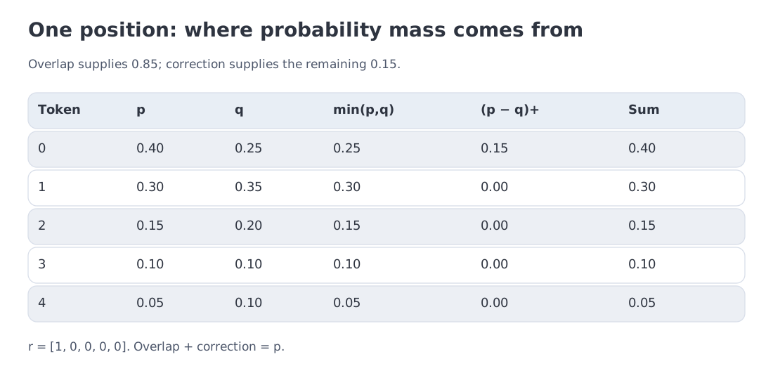 The overlap, residual mass, and exact reconstruction of the target distribution for the five-token example.
Two boundary cases deserve explicit tests. When , rejection cannot occur and no residual distribution is needed. When , the ratio should never be evaluated: the proposer cannot emit token , and any missing target mass is recovered through the residual.
NumPy → PyTorch · B18 — Exact speculative correction
NumPy exposes overlap mass and the positive residual (p-q)+. PyTorch uses the same balance and torch.multinomial; tests pass a dedicated random generator.
import numpy as np
import torch
1. Explicit NumPy implementation
def numpy_rejection_kernel_explicit(
    p: np.ndarray,
    q: np.ndarray,
) -> tuple[np.ndarray, np.ndarray, np.ndarray]:
    acceptance = np.zeros_like(p, dtype=np.float64)
    support = q > 0
    acceptance[support] = np.minimum(1.0, p[support] / q[support])
    overlap = np.minimum(p, q)
    positive = np.maximum(p - q, 0.0)
    residual_mass = positive.sum()
    residual = positive / residual_mass if residual_mass > 0 else np.zeros_like(p)
    reconstructed = overlap + residual_mass * residual
    return acceptance, residual, reconstructed
NumPy exposes all three parts of the proof: acceptance min(1,p/q), overlap min(p,q), and the normalized positive residual (p-q)_+.
2. The same mathematics as explicit PyTorch operations
def torch_rejection_kernel_explicit(
    p: torch.Tensor,
    q: torch.Tensor,
) -> tuple[torch.Tensor, torch.Tensor, torch.Tensor]:
    acceptance = torch.zeros_like(p)
    support = q > 0
    acceptance[support] = torch.minimum(torch.ones_like(p[support]), p[support] / q[support])
    overlap = torch.minimum(p, q)
    positive = torch.clamp(p - q, min=0)
    residual_mass = positive.sum()
    residual = positive / residual_mass if bool(residual_mass > 0) else torch.zeros_like(p)
    reconstructed = overlap + residual_mass * residual
    return acceptance, residual, reconstructed

def torch_sample_speculative_token_explicit(
    p: torch.Tensor,
    q: torch.Tensor,
    proposal: int,
    *,
    generator: torch.Generator | None = None,
) -> tuple[int, bool]:
    if isinstance(proposal, bool) or not isinstance(proposal, int) or not 0 <= proposal < p.numel() or q[proposal] <= 0:
        raise ValueError("proposal must be an integer in the positive support of q")
    acceptance, residual, _ = torch_rejection_kernel_explicit(p, q)
    draw = torch.rand((), generator=generator, device=p.device, dtype=p.dtype)
    if draw < acceptance[proposal]:
        return int(proposal), True
    return int(torch.multinomial(residual, 1, generator=generator).item()), False
The explicit kernel assumes matching one-dimensional p and q vectors with at least two entries: finite, nonnegative, and normalized. Torch inputs share one device and a common float32 or float64 dtype. It normalizes positive differences without discarding a small residual. Sampling is an inference operation; discrete choices do not carry an ordinary gradient. The optional generator defaults to the global RNG; tests pass a separate torch.Generator for reproducibility. The proposal must have been sampled from q, not supplied arbitrarily.
| Aspect | NumPy | PyTorch |
|---|---|---|
| Support of q | explicit q>0 mask | boolean tensor mask |
| Acceptance | np.minimum | torch.minimum |
| Residual | np.maximum(p-q,0) | torch.clamp(..., min=0) |
| Sampling | outside the mathematical kernel | torch.rand / multinomial with a generator |
| Test | exact reconstruction of p | Monte Carlo plus algebraic parity |
Executable parity and edge-case check
p_np = np.array([0.40,0.30,0.15,0.10,0.05]); q_np = np.array([0.25,0.35,0.20,0.10,0.10])
a_np, r_np, b_np = numpy_rejection_kernel_explicit(p_np, q_np)
a_t, r_t, b_t = torch_rejection_kernel_explicit(torch.tensor(p_np), torch.tensor(q_np))
np.testing.assert_allclose(a_np, a_t.numpy()); np.testing.assert_allclose(r_np, r_t.numpy()); np.testing.assert_allclose(b_np, b_t.numpy()); np.testing.assert_allclose(b_np, p_np)
gen = torch.Generator().manual_seed(18); counts = torch.zeros(5)
q = torch.tensor(q_np); p = torch.tensor(p_np)
for _ in range(12000):
    proposal = int(torch.multinomial(q, 1, generator=gen))
    token, _ = torch_sample_speculative_token_explicit(p, q, proposal, generator=gen)
    counts[token] += 1
assert torch.max(torch.abs(counts / counts.sum() - p)) < 0.02

# A real, tiny residual must remain a probability distribution.
near_q = np.array([1.0, 0.0]); near_p = np.array([1.0-1e-14, 1e-14])
for kernel, args in [
    (numpy_rejection_kernel_explicit, (near_p, near_q)),
    (torch_rejection_kernel_explicit, (torch.tensor(near_p), torch.tensor(near_q))),
]:
    _, residual, balance = kernel(*args)
    np.testing.assert_allclose(np.asarray(residual), [0.0, 1.0], rtol=0, atol=1e-15)
    np.testing.assert_allclose(np.asarray(balance), near_p, rtol=0, atol=1e-15)
# Uniform RNG can return zero: a zero-acceptance proposal must still be rejected.
from unittest.mock import patch
with patch.object(torch, "rand", return_value=torch.tensor(0.0, dtype=torch.float64)):
    token, accepted = torch_sample_speculative_token_explicit(
        torch.tensor([0.,1.], dtype=torch.float64),
        torch.tensor([1.,0.], dtype=torch.float64), 0, generator=gen)
    assert token == 1 and not accepted

print("B18 exact balance, tiny residual, zero draw, Monte Carlo: PASS")
Complete executable file: m11_inference_bridges.py
6. Expected progress per cycle
A compact model assumes conditional acceptance probability for each next proposal, given that every earlier proposal survived. This is a modelling assumption about each reached position, not a consequence of knowing an overall acceptance average. Actual conditional rates can vary with prompt, position, and proposed history; Section 7 shows why their average is insufficient.
Every cycle emits at least one token. It emits a second token if the first proposal is accepted, a third if the first two are accepted, and so on. Thus
For ,
for , the finite sum is simply .
At and , the expectation is 2.94 tokens. At and , it is 5.70. Assuming the previous example’s applies conditionally at every reached position gives 3.71 tokens for .
The diminishing return is visible in the limiting value . A longer proposal is useful only if the probability of reaching its later positions is high enough. This is why proposer quality and cost dominate naïve “more speculative tokens” tuning.
7. A cost model, an optimum, and an illustrative MTP point
The general progress expression is a tail sum. Let mean that the first proposals were accepted. Then With , we have . Two conditional rates, 0.9 and 0.5, give emitted tokens. Replacing them with their average, 0.7, gives 2.19. A mean acceptance rate alone therefore does not determine mean cycle length.
Expected tokens are not elapsed time. Let denote the cost of one draft step relative to one target step. A transparent first-order scenario is
The denominator assumes that block verification costs one ordinary target step. A measured model can use instead, where is verification time and other overhead, in the same units. Exactness makes no claim about these costs. Include ordinary decoding, and normalized speed 1, when choosing a method: every positive proposal length may be slower.
This expression is intentionally incomplete. Tree construction, KV movement, launch overhead, batching, and a non-linear verification cost are outside it. Its value is conceptual: it exposes the tradeoff between more accepted work and more proposal work.
Second pass: should the draft grow by one token? Holding and fixed gives . Comparing adjacent speed ratios yields The right-hand side converts the extra proposal time into tokens at the current rate. Comparing the output increment directly with would mix an expected token count with a time cost. The notebook exercise checks this condition against a full scan.
With and , scanning gives the maximum at :
The optimum is broad rather than sharp. gives 2.46, while still gives 2.35. In practice, reducing proposer cost or improving overlap often matters more than choosing the last decimal of proposal length.
Now take an illustrative native-MTP scenario with one proposed token: , , and . Then
The 1.79× result belongs to these chosen parameters. It is not a derivation of a vendor benchmark. It is a useful calibration: a cheap, high-acceptance, one-step proposer can plausibly produce a gain of that order, while enforces the simple upper bound .
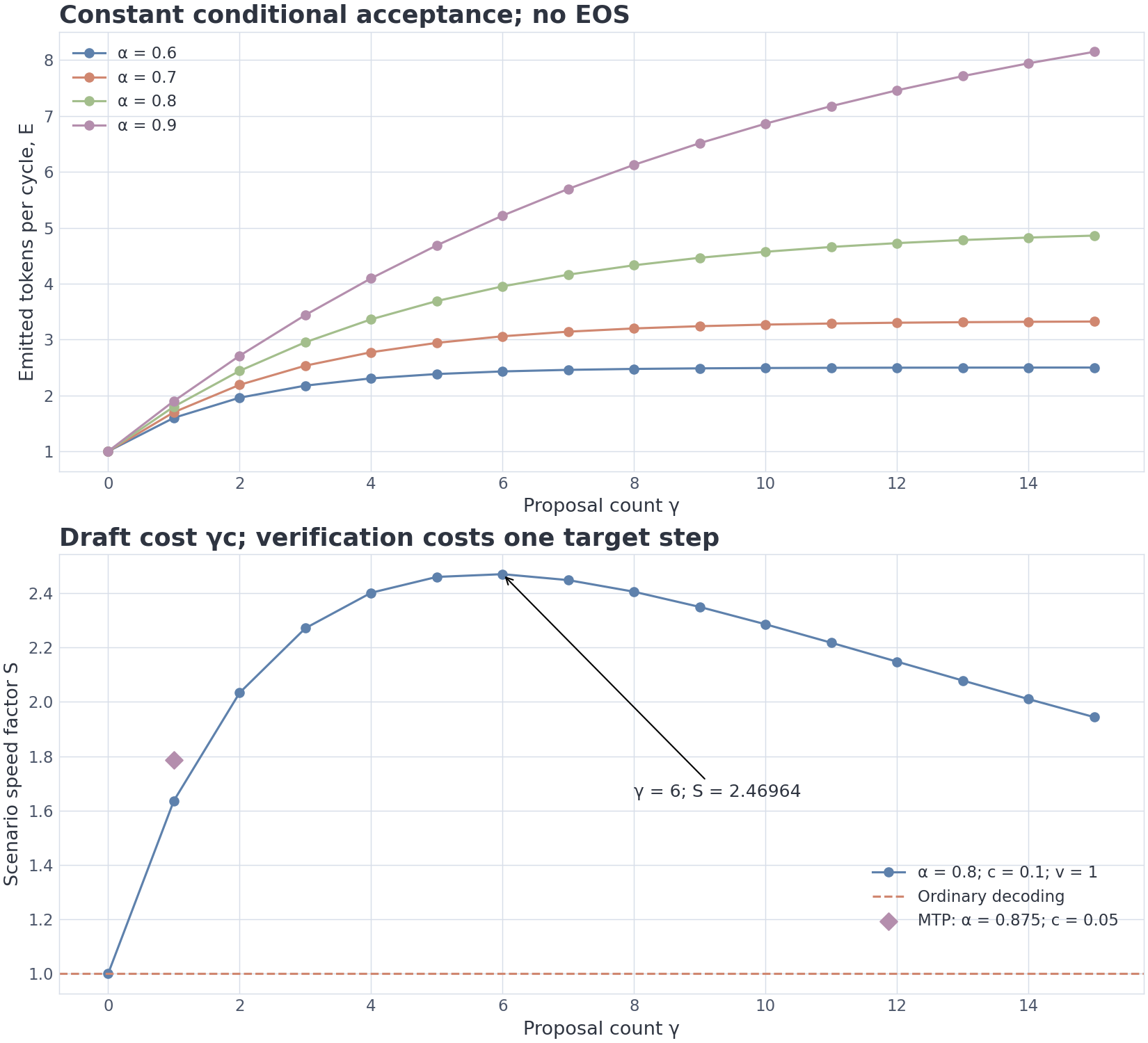 Expected cycle length saturates with proposal length; the scenario speed curve has a broad optimum. The MTP marker is an illustrative parameter point.
A fixed is only a baseline. An online system can adapt proposal length to confidence, domain, current load, and measured verification efficiency.
8. A taxonomy of proposers
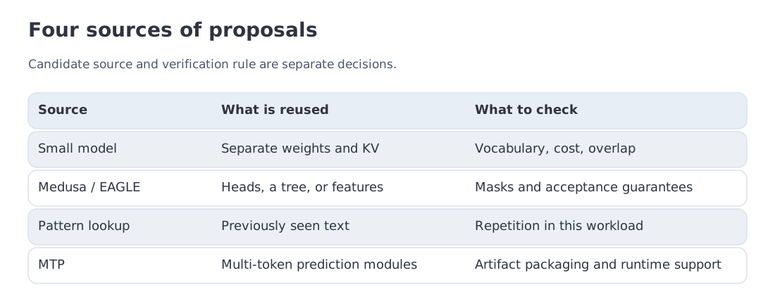 External draft models, auxiliary-head and EAGLE-style proposers, pattern lookup, and native MTP occupy different points in the cost–overlap–complexity space.
A separate draft model is the cleanest reference design. A smaller sibling proposes a linear continuation, and the large model verifies it. The operational costs are a second set of weights, additional KV state, and a possible distribution mismatch. Tokenizer compatibility is part of the design, not an afterthought.
Auxiliary heads and candidate trees trade model size for structured proposals. Medusa predicts several offsets and verifies a tree. Its typical-acceptance scheme aims to preserve useful generation quality; that criterion does not automatically provide the exact stochastic guarantee from Section 4. A wider tree can raise the chance that a useful path survives, but it changes mask construction, candidate selection, and verification cost.
EAGLE-family proposers learn from target-model features. EAGLE-3 replaces feature regression with direct token prediction and fuses representations from multiple layers. Its paper reports speedups up to 6.5× in the authors’ test settings and, separately, a 1.38× SGLang throughput gain at batch size 64. That is evidence that the design can be powerful, not a portable constant for every engine and workload.
Lookup-based methods propose text already present in the prompt, generated history, or a suffix structure. They can be remarkably effective for code, document extraction, and repeated templates because the proposal cost is low and literal continuation is common. Their usefulness falls when answers are novel rather than copied or patterned.
Native MTP reuses prediction capacity built into the target architecture. It removes the need to select and serve a separate full draft model. It does not remove the need to measure acceptance, additional memory, and verifier efficiency.
No universal batch-size cutoff separates winning and losing regimes. Current vLLM guidance positions speculative decoding primarily as an inter-token-latency optimization for memory-bound workloads at medium-to-low query rates (QPS means queries per second). Once ordinary batching saturates compute, proposal work may compete with useful target work.
9. Native multi-token prediction at inference time
Multi-token prediction is first a training objective. The model is asked to predict more than the immediate next token, which may require auxiliary heads, extra blocks, or shared-weight modules. Whether those components remain available at inference is an architectural and checkpoint decision.
The DeepSeek-V3 technical report states that its MTP objective can be used for speculative decoding. The report does not turn that sentence into a universal acceptance rate or speedup. A deployment still needs a retained proposer, a compatible runtime implementation, and workload-specific measurements.
Current vLLM documentation describes MTP as a speculative mode for models with native multi-token capability. The usual native path needs no separate full draft model. Packaging is architecture-specific: the documented Gemma 4 MTP path takes a compatible assistant checkpoint, while other families retain the modules in the main artifact.
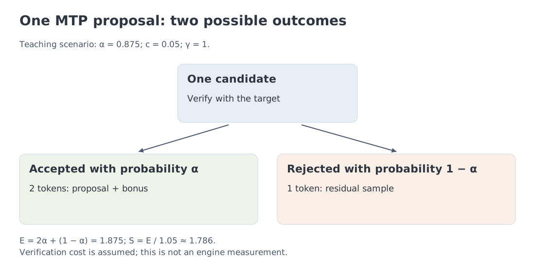 A native MTP module proposes future tokens from the target model’s own representation; the target trunk verifies them. The 1.79× value is explicitly a teaching scenario.
A one-token native proposer is operationally attractive but mathematically capped at two emitted tokens per cycle. Multi-step and recursive proposers relax that cap at the price of extra work and more complicated error propagation. The right comparison is therefore multidimensional: accepted length, proposal latency, verification latency, memory overhead, and behavior under concurrency.
Speculation is also relevant inside RL post-training. A rollout is a generated response or action trajectory that will be evaluated and used for learning. Generating this experience can dominate the wall-clock budget, and exact target-preserving speculation can accelerate that stage without changing the policy distribution being sampled. Module 12 of RL for LLM develops the surrounding actor/learner, worker, and asynchronous infrastructure; this lecture supplies one possible inference primitive inside that system.
10. Verification as a short, wider decode operation
Ordinary decode evaluates one new position. Verification evaluates several proposed positions together. The matrix operations become wider, so the target performs more useful arithmetic per weight read. Calling this a “mini-prefill” is an intuition about arithmetic intensity, not an identity between the two phases.
Using the same simple speed scenario, take , , and . The multiplier is 2.83790769. Applied to the 209.4 token/s weight-only bf16 ceiling,
The number is an arithmetic what-if. It assumes that one target verification is close to one target decode read and that weight bandwidth remains the bottleneck. KV traffic, wider activation work, tree masks, scheduling, and kernel efficiency all reduce or reshape the gain.
The system metric also matters. Speculation may improve inter-token latency for a single request while leaving saturated-server goodput unchanged—or even lower. Here inter-token latency (ITL) is the interval between delivered tokens; goodput counts only work meeting the chosen quality and latency requirements. A credible evaluation reports per-request throughput, ITL, and aggregate goodput over a concurrency sweep.
11. What low-bit quantization actually changes
Start with a numerical mechanism. For a symmetric integer group, choose , store , and reconstruct . Codes are dimensionless; the scale restores the original units and range. A large scale accommodates outliers but leaves coarse spacing near zero. A small scale resolves common values more finely while clipping extremes.
For a layer , weight error becomes output error through . An error on a frequently active input channel can matter more than the same error elsewhere. A calibration set is a small collection of representative inputs used to estimate that sensitivity before deployment.
“Four-bit model” is a marketing shorthand, not a complete numerical specification. A deployment must say which tensors are quantized, how scales are stored, what precision is used for accumulation, and whether the hardware executes the representation natively.
Post-training quantization (PTQ) transforms a trained checkpoint. Its weight-only form reduces model weights while keeping activations and accumulation at higher precision. W8A8 and W4A4 also reduce activations. Quantization-aware training (QAT) exposes the model to quantization effects during training. Many PTQ methods use calibration data, although direct rounding can be data-free. W names weights and A activations; the numerals in W4A4 specify their representation widths. Accumulation precision remains a separate choice.
GPTQ quantizes weights while accounting for how local weight error affects a layer’s output. AWQ uses activation statistics to protect channels that matter disproportionately. Neither method should be judged solely by weight MSE: the relevant outcome is the model’s logits, calibration, and downstream quality.
For parameters at an effective bits per weight,
The module’s 8B accounting is:
| representation | effective bits/weight | decimal GB | weight-stream ceiling at 3.35 TB/s |
|---|---|---|---|
| bf16 | 16.00 | 16.00 | 209.38 tok/s |
| FP8 | 8.00 | 8.00 | 418.75 |
| NVFP4-like accounting | 4.50 | 4.50 | 744.44 |
| MXFP4-like accounting | 4.25 | 4.25 | 788.24 |
| idealized W4 | 4.00 | 4.00 | 837.50 |
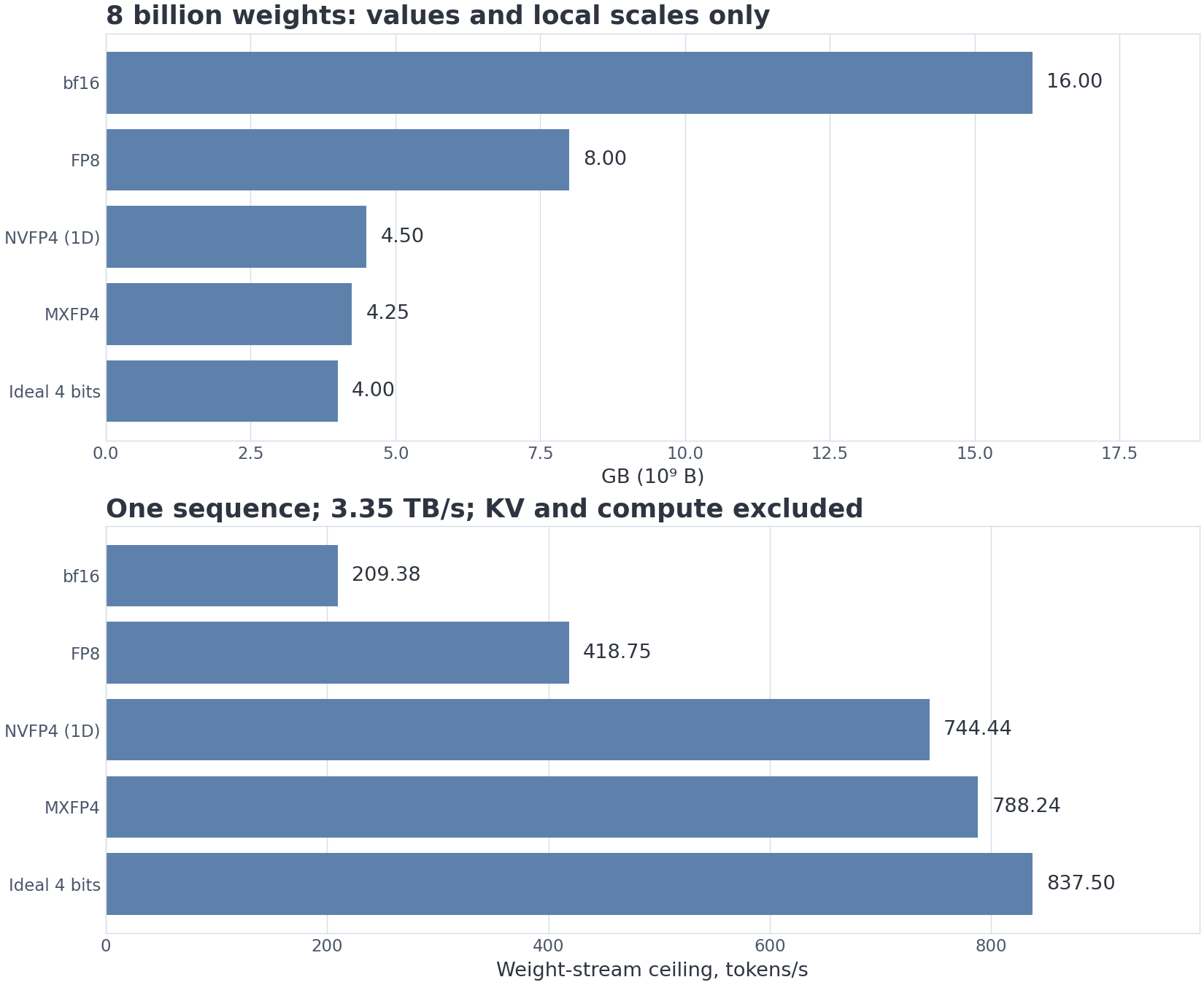 An arithmetic payload ladder. The 4.50- and 4.25-bit entries include local scales. Additional metadata, alignment, unquantized tensors, and format-specific packing are excluded.
The table is useful precisely because it is narrow. It says what happens to a weight-read ceiling when payload changes. It says nothing yet about accuracy, dequantization, KV cost, or achieved bandwidth.
12. Microscaled FP4, W4A4, and the role of hardware
E2M1 allocates one sign bit, two exponent bits, and one fraction bit. Its spacing is nonuniform. Available magnitudes are ; positive and negative zero give 16 encodings but 15 distinct values. The teaching quantizer stores those 15 values. E4M3 is an eight-bit floating-point format with four exponent bits and three fraction bits. The E8M0 scale in MX encodes a power of two, with no fraction field.
Four bits provide very few numerical levels. A single scale for an entire tensor would either waste resolution around zero or clip outliers. Microscaling assigns a local scale to a small group of low-bit values.
NVIDIA documents NVFP4 as E2M1 values with hierarchical block scaling. In the one-dimensional recipe, a block of 16 values shares an E4M3 scale and the tensor has an additional FP32 global scale. Counting only the local eight-bit scale gives
The actual training recipe may use different geometry for weights, including 16×16 blocks, and a concrete checkpoint has additional metadata and unquantized tensors.
MXFP4 is commonly represented as 32 E2M1 values sharing an E8M0 scale:
The lower metadata rate does not imply universally better performance. Scale expressiveness, block granularity, calibration, and native kernel support determine the quality–speed tradeoff.
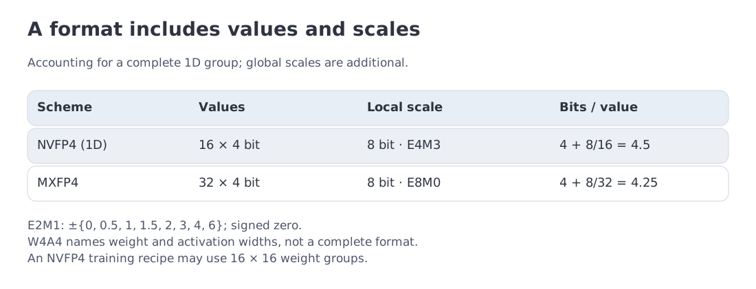 NVFP4 and MXFP4 use different local-scale schemes. W4A4 adds activation quantization; ternary models require a still more specialized training and execution path.
MR-GPTQ is a useful corrective to simplistic format rankings. The authors adapt PTQ to microscaled floating-point formats, report substantial quality and hardware-speed improvements in their setups, and explicitly conclude that FP4 is not an automatic upgrade over INT4.
W4A4 moves beyond weight compression. Cohere reports that Command A+, a 218B-total/25B-active MoE model, can run at W4A4 on one B200 or two H100s. That claim belongs to the released model, its calibration, and its supported software path. It should not be generalized to an arbitrary 218B model.
The notebook’s E2M1-like example compares two toy quantizers on one vector containing an outlier. Symmetric INT4 has 3.32 times the MSE of the teaching FP4 grid for that vector. The experiment demonstrates a range-allocation effect; it is not a cross-model benchmark.
BitNet-style ternary weights push the representation much further. Their potential benefit depends on co-designed training, packing, and kernels. A tiny checkpoint representation alone does not create ternary arithmetic on conventional accelerators.
13. Code: make the probability contract explicit
The first function below validates the exact mass balance for one speculative position. The second is a grouped E2M1-like teaching quantizer. It is not a bit-exact NVFP4 implementation and contains no packed storage or GPU kernel.
"""M11 minimal probability and grouped-value teaching kernels."""
import numpy as np

def probability_vector(values, *, name="p", atol=1e-12):
    """Validate a distribution without hidden clipping or renormalization."""
    x = np.asarray(values, dtype=np.float64)
    if x.ndim != 1 or x.size < 2 or not np.isfinite(x).all():
        raise ValueError(f"{name}: expected a finite one-dimensional vector")
    if np.any(x < 0) or not np.isclose(x.sum(), 1.0, rtol=0.0, atol=atol):
        raise ValueError(f"{name}: probabilities must be >= 0 and sum to 1")
    return x

def rejection_kernel(p_values, q_values):
    """Acceptance probabilities, residual, and exact one-position balance."""
    p = probability_vector(p_values, name="p")
    q = probability_vector(q_values, name="q")
    if p.shape != q.shape:
        raise ValueError("p and q must use the same vocabulary")

    acceptance = np.zeros_like(p)
    support = q > 0  # q_t=0 means the proposer cannot emit token t
    acceptance[support] = np.minimum(1.0, p[support] / q[support])

    overlap = np.minimum(p, q)
    positive = np.maximum(p - q, 0.0)
    residual_mass = positive.sum()
    residual = (
        positive / residual_mass
        if residual_mass > 0.0
        else np.zeros_like(p)
    )
    balance = overlap + residual_mass * residual
    np.testing.assert_allclose(balance, p, rtol=0.0, atol=1e-12)
    return acceptance, residual, balance

def quantize_grouped_e2m1(values, group_size=16):
    """Teaching E2M1-like grid with one scale per group."""
    grid = np.array(
        [-6, -4, -3, -2, -1.5, -1, -0.5, 0,
          0.5, 1, 1.5, 2, 3, 4, 6],
        dtype=np.float64,
    )
    x = np.asarray(values, dtype=np.float64)
    if x.ndim != 1 or x.size == 0 or not np.isfinite(x).all():
        raise ValueError("expected a non-empty finite one-dimensional vector")
    if isinstance(group_size, bool) or not isinstance(group_size, (int, np.integer)) or group_size <= 0 or x.size % group_size:
        raise ValueError("length must be divisible by a positive group_size")

    groups = x.reshape(-1, group_size)
    max_abs = np.max(np.abs(groups), axis=1, keepdims=True)
    scale = np.where(max_abs > 0, max_abs / 6.0, 1.0)
    normalized = groups / scale
    codes = np.abs(normalized[..., None] - grid).argmin(axis=-1)
    return (grid[codes] * scale).reshape(x.shape)
The validator deliberately refuses to normalize malformed probability vectors. Silent repair would hide an error in the sampling algorithm. The quantizer treats an all-zero group explicitly so that a zero scale cannot produce NaNs.
A production implementation must add vectorized batches, a specified rounding rule, packed storage, scale metadata, format-compatible matrix kernels, and device-level tests.
NumPy → PyTorch · B19 — Grouped fake quantization
Groups are formed only along the last dimension, so values from different experts never share a scale.
import numpy as np
import torch
import torch.nn.functional as F
1. Explicit NumPy implementation
def numpy_grouped_fake_quant_explicit(
    x: np.ndarray,
    *,
    grid: np.ndarray,
    group_size: int,
) -> np.ndarray:
    pad = (-x.shape[-1]) % group_size
    padded = np.pad(x, [(0, 0)] * (x.ndim - 1) + [(0, pad)])
    groups = padded.reshape(*x.shape[:-1], -1, group_size)
    max_abs = np.max(np.abs(groups), axis=-1, keepdims=True)
    scales = np.where(max_abs > 0, max_abs / np.max(np.abs(grid)), 1.0)
    normalized = groups / scales
    codes = np.abs(normalized[..., None] - grid).argmin(axis=-1)
    return (grid[codes] * scales).reshape(padded.shape)[..., : x.shape[-1]]
NumPy pads only the last dimension, forms groups, computes a local scale, and selects the nearest grid value. Leading axes—such as expert index—never share a group.
2. The same mathematics as explicit PyTorch operations
def torch_grouped_fake_quant_explicit(
    x: torch.Tensor,
    *,
    grid: torch.Tensor,
    group_size: int,
) -> torch.Tensor:
    grid = grid.to(device=x.device, dtype=x.dtype)
    pad = (-x.shape[-1]) % group_size
    padded = torch.nn.functional.pad(x, (0, pad)) if pad else x
    groups = padded.reshape(*x.shape[:-1], -1, group_size)
    max_abs = groups.abs().amax(dim=-1, keepdim=True)
    scales = torch.where(max_abs > 0, max_abs / grid.abs().max(), torch.ones_like(max_abs))
    normalized = groups / scales
    codes = (normalized[..., None] - grid).abs().argmin(dim=-1)
    return (grid[codes] * scales).reshape(padded.shape)[..., : x.shape[-1]]
The explicit kernel assumes finite real floating arrays with nonempty axes; use float32/float64 for parity. Group size is a positive integer. The grid is a finite one-dimensional array containing exact zero and a nonzero level, including after conversion to the input dtype. Intermediate scales and distances must be representable in that working dtype. PyTorch repeats reshape, amax, broadcasting, and argmin. This is fake quantization: the result remains an ordinary tensor, without packed bits. Ties select the first grid entry; this teaching rule does not implement every hardware rounding mode.
| Aspect | NumPy | PyTorch |
|---|---|---|
| Grouping | reshape the last axis | same reshape |
| Padding | np.pad | F.pad |
| Scale | max_abs / max_grid | same tensor expression |
| Code | argmin over the grid | argmin(dim=-1) |
| Result | dequantized array | dequantized tensor, not packed bits |
Executable parity and edge-case check
rng = np.random.default_rng(19)
x_np = rng.standard_normal((3,2,11))
grid_np = np.array([-6,-4,-3,-2,-1.5,-1,-0.5,0,0.5,1,1.5,2,3,4,6.0])
np_q = numpy_grouped_fake_quant_explicit(x_np, grid=grid_np, group_size=4)
t_q = torch_grouped_fake_quant_explicit(torch.tensor(x_np), grid=torch.tensor(grid_np), group_size=4)
np.testing.assert_allclose(np_q, t_q.numpy())
zeros = torch.zeros(2,3,7, dtype=torch.float64)
zero_q = torch_grouped_fake_quant_explicit(zeros, grid=torch.tensor(grid_np), group_size=4)
torch.testing.assert_close(zero_q, zeros)
print("B19 explicit grouped fake quantization: PASS")
Complete executable file: m11_inference_bridges.py
15. Combining the levers without multiplying away the bottlenecks
The concepts compose cleanly. Quantization lowers the target payload; speculation amortizes a target invocation over more emitted tokens. The module’s narrow arithmetic model can therefore combine them.
An 8B model at 4.5 GB has a weight-only ceiling of 744.44 tokens/s at 3.35 TB/s. Applying the illustrative MTP multiplier from Section 7 gives
That is 6.35 times the bf16 weight-only baseline. It is not a predicted end-to-end result. The calculation omits KV traffic, quantization/dequantization overhead, extra proposer parameters, scheduling, and the possibility that the system becomes compute-bound.
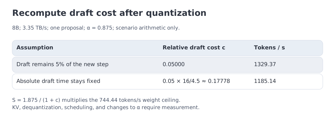 Two scenarios differ in whether drafting becomes cheaper alongside the target. Recompute c relative to the new target step before combining estimates.
Quantization can also change target logits, so the acceptance statistics must be remeasured after quantization.
Relative cost needs the same care. If the target becomes times faster but draft time stays fixed, normalized draft cost rises from to . For , an original becomes 0.17778. Keeping acceptance at 0.875 then gives about 1185.14 tokens/s, rather than 1329.37, in the same simplified model. The higher figure assumes that drafting remains five percent of the new target step. Exact speculative sampling still matches the deployed target distribution, but that distribution may differ from the high-precision model.
QLoRA belongs to the same broad economy of low-bit storage but solves a different problem. It freezes a four-bit base model and trains higher-precision low-rank adapters, reducing fine-tuning memory. It is neither a quantized inference kernel nor a speculative sampler.
For a deeper conceptual view, Module 9 of Information Theory for ML develops rate–distortion reasoning, and Module 14 discusses why local quantization error is not a complete task-level distortion measure. Those references are optional; the present module contains all formulas needed for its own conclusions.
16. A deployment workflow for current engines
Define the outcome before benchmarking. TTFT is time to first token; ITL is the interval between subsequent delivered tokens. Throughput counts work per unit time. Goodput counts work meeting specified quality and latency requirements, often expressed as service-level objectives (SLOs). A server can produce more tokens overall while delivering fewer acceptable responses before their deadlines.
As of October 11, 2026, vLLM documents several speculative families: external draft models, EAGLE, native MTP, n-gram and suffix proposal, plus specialized variants. Its guidance frames speculation primarily as an inter-token-latency optimization for memory-bound, medium-to-low-QPS workloads.
A reliable rollout starts from a controlled baseline. Pin the model revision, tokenizer, engine and kernel versions, GPU type, sampling configuration, prompt/output distributions, and concurrency. Measure quality, memory, TTFT, ITL, throughput, and goodput.
Next, introduce quantization alone. Confirm that the runtime is using the intended kernel rather than merely storing a compressed checkpoint. Re-run quality and performance tests.
Then add speculation alone. Record proposer cost, mean accepted length, rejection rate, verification time, and memory overhead. Finally, combine the two and re-profile from scratch. This sequence reveals which technique moved the bottleneck and prevents crediting one component for another component’s gain.
For native MTP, check whether proposal modules are bundled in the target or distributed as a compatible auxiliary artifact; the runtime must recognize that architecture. EAGLE and generic draft-model modes require compatible artifacts. Lookup methods require favorable text structure rather than a neural checkpoint.
The success criterion depends on the product. Interactive chat emphasizes TTFT, ITL, and tail latency. Offline generation values aggregate goodput. RL rollouts care about accepted samples per training-hour and the interaction with asynchronous worker scheduling.
17. Reading a quant/spec run passport
A reproducible result should be expressible as a passport rather than a slogan.
Target: exact checkpoint revision, tokenizer, sampling policy, context limit, attention/KV representation, and any model-side speculative modules.
Quantization: tensors quantized, value format, group geometry, local and global scale types, calibration method and data, accumulation precision, excluded layers, kernel version, and hardware support.
Proposer and verifier: proposer family and checkpoint, native MTP configuration if applicable, proposal length or tree shape, tokenizer compatibility, acceptance rule, mean accepted length by task family, proposal time, and verification time.
Workload: prompt and output length distributions, concurrency/QPS, batch policy, temperature/top-p, repetition structure, and SLO.
Outcomes: TTFT, ITL, per-request throughput, aggregate goodput, memory footprint, quality metrics, tail percentiles, date, and complete software/hardware versions.
A group size of 16 does not uniquely identify NVFP4. A filename suffix does not prove that the corresponding kernel executed. The artifact, configuration, and runtime path must agree.
20. What to retain and sources
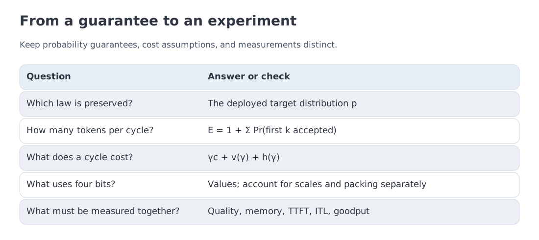 Exact sampling equations, cycle economics, proposer families, low-bit accounting, and the deployment checklist on one page.
Exact speculative sampling uses a cheap proposal without replacing the target distribution:
Assuming the same conditional acceptance probability at each reached position,
but elapsed-time benefit depends on proposal and verification cost. is a teaching model and an initial sanity check, not a runtime contract.
Quantization is a format-plus-scaling-plus-kernel decision. FP4 is not automatically superior to INT4, W4A4 is not automatically safe, and weight MSE is not a complete quality metric.
When quantization and speculation are combined, acceptance and bottlenecks must be remeasured. Speedups reported under different hardware, concurrency, and precision settings are not independent factors.
Primary references:
- Leviathan, Kalman, and Matias — Fast Inference from Transformers via Speculative Decoding.
- Cai et al. — Medusa.
- Li et al. — EAGLE and EAGLE-3.
- DeepSeek-AI — DeepSeek-V3 Technical Report.
- Frantar et al. — GPTQ.
- Lin et al. — AWQ.
- Dettmers et al. — QLoRA.
- Egiazarian et al. — MR-GPTQ.
- NVIDIA Transformer Engine — NVFP4 format and scaling.
- OCP — Microscaling Formats (MX), version 1.0.
- vLLM — Speculative Decoding and MTP.
- Cohere — Command A+.
Optional deepening: rate–distortion and model quantization appear in Modules 9 and 14 of Information Theory for ML. Rollout-generation cost and asynchronous RL infrastructure are developed in Module 12 of RL for LLM.
Module 12 changes the generation protocol itself: a diffusion model refines several positions per pass. We will compare it with the autoregressive and speculative methods developed here before returning to SFT and post-training data in Module 13.
Landscape verified: October 11, 2026. Claims about engines, formats, and releases were verified against primary sources. The module’s weight-stream and speed calculations are explicit scenarios; external results are attributed to their sources and experimental settings.