Module 12. Diffusion Language Models
Modern LLMs · Module 12 lecture · 11 October 2026 edition
What this module changes. We have built and trained an autoregressive model, studied its serving costs, and seen how speculative decoding can accelerate generation while preserving its target distribution. Here the architecture can remain recognizably Transformer-like while the generation protocol changes. An autoregressive (AR) model commits one token at a time. A diffusion large language model (dLLM) starts from a corrupted draft and repeatedly predicts many positions. The working sequence is called a canvas; recovering its tokens is denoising. We will derive the absorbing-mask objective, execute a transparent denoising trace, examine reveal and remasking policies, and build a deliberately generic 8B roofline scenario. Only after that will we read the actual DiffusionGemma passport, keeping a teaching bound separate from a released system measurement.
Prerequisites. We build on autoregressive generation from Module 3, pretraining from Module 9, the serving cost model from Module 10, and speculative decoding from Module 11. Together they make a fair comparison of generation protocols possible. The sparse-model discussion also uses MoE from Module 7.
First pass: read Sections 1 and 4–9 for the mechanism, Section 10 for one cost calculation, and Section 14 for block generation. In Section 7, focus on what the loss measures and the worked example; return to the expectation formula later. Use Section 18 to check your understanding.
Second pass: work through the objective in Section 7, batching in Section 11, and the implementation in Sections 12–13 before doing the notebook and Section 19 exercises. Reference pass: Sections 2–3 explain the origins of the ideas; Sections 15–17 are a dated guide to released systems.
Contents
- The sequential unit of work
- How the field arrived here
- Three intellectual ancestors
- A two-axis map
- The absorbing-mask forward process
- Worked example A: a mask schedule
- Training objective and likelihood
- Any-order training and its limits
- Sampling and worked example B
- A generic roofline calculation
- Steps, batching, and weight precision
- Level-1 code
- What the notebook verifies
- Block diffusion, length, and caching
- Reading the DiffusionGemma passport
- The dLLM landscape on 11 October 2026
- Multimodal diffusion systems
- Self-check questions
- Exercises
- Takeaways and sources
1. The sequential unit of work
The bottleneck in batch-one autoregressive decoding is often not a shortage of arithmetic. The problem is that a very large set of weights is streamed for one incremental token. The model then waits for that token before the next decode step can begin.
Take a deliberately stripped-down scenario: an 8-billion-parameter dense model, 16 GB of bf16 weights, 3.35 TB/s of memory bandwidth, and a 990-TFLOP/s arithmetic peak. A weight-stream lower bound for one decode step is
The corresponding ideal matrix arithmetic would take only
The ratio , 0.338%, is not a measured GPU-utilization number. It is the share of this simplified step lower bound occupied by ideal arithmetic. Under these assumptions the batch-one ceiling is 209.375 tokens/s.
A diffusion sampler changes the granularity. One network invocation scores an entire canvas of positions. The price is denoising calls rather than one causal call per token. The rough arithmetic becomes
For , one ideal pass costs 16.549 ms of compute and is no longer limited by the 4.776-ms weight stream. At , the arithmetic ceiling is 966.8 tokens/s—4.62 times the batch-one AR ceiling, despite roughly 64 times more FLOPs.
This apparent paradox is the core engineering proposition of diffusion decoding: do more total work, but cross fewer sequential barriers. It is only a proposition, not a guaranteed result. Bidirectional attention over the canvas, activation traffic, MoE expert union, kernel quality, runtime overhead, and the number of useful denoising steps determine whether the trade pays off.
There is also a behavioral distinction. A masked-diffusion sampler can reopen a weak position and revise it in the next iteration. A standard ancestral AR decode does not revise its committed prefix. AR systems can of course add a verifier, a second editing pass, Fill-in-the-Middle (FIM), or an agent loop; diffusion places revision inside the sampling algorithm itself.
2. How the field arrived here
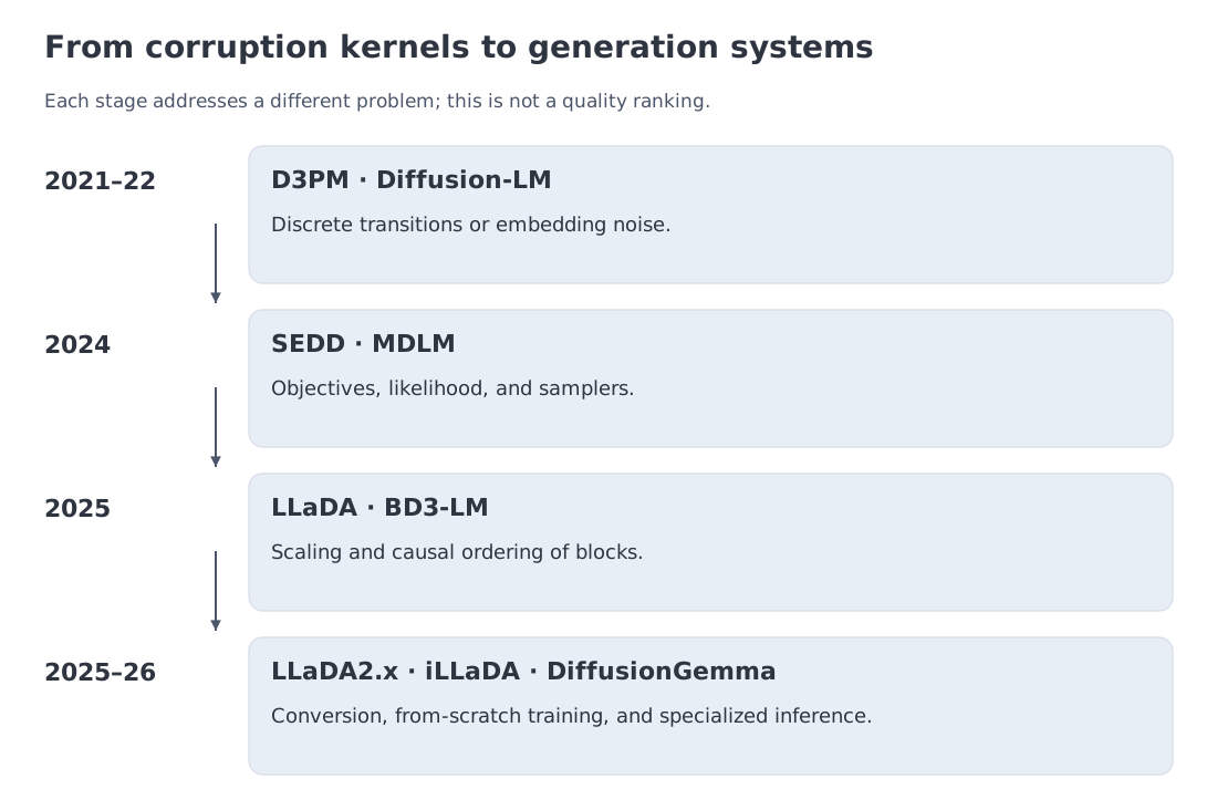 The line from discrete transition kernels to masked likelihood models, block diffusion, open-weight systems, and commercial APIs. Each milestone addresses a different obstacle rather than replacing all earlier methods.
The first problem was mathematical: what does “add noise” mean when the object is a token ID? D3PM — Discrete Denoising Diffusion Probabilistic Models (2021) answered with transition matrices over discrete states. One option was an absorbing state: a token may become [MASK] and remains masked in the forward process.
Diffusion-LM (2022) explored a continuous alternative. It corrupted token embeddings with Gaussian noise and later rounded the resulting representation back to the vocabulary. The route offered controllability, but the continuous-to-discrete boundary added its own difficulty.
By 2024, discrete objectives became much more competitive. SEDD — Score Entropy Discrete Diffusion developed a suitable discrete score objective. MDLM — Masked Diffusion Language Models showed that an absorbing-mask construction admits a simple likelihood-oriented loss and efficient samplers, including semi-autoregressive variable-length generation.
Scale became the next question. LLaDA 8B was trained from scratch on 2.3T tokens. BD3-LM introduced block diffusion, letting completed blocks form a causal prefix while the active block is denoised bidirectionally. LLaDA-MoE, Dream, Seed Diffusion, Mercury, and Gemini Diffusion explored sparse models, AR-checkpoint conversion, and specialized runtimes.
The 2025–2026 wave broadened both routes. LLaDA2.0 converted 16B and 100B AR-MoE checkpoints through a Warmup–Stable–Decay (WSD) schedule. LLaDA2.1 added Token-to-Token correction so already revealed values could be replaced. iLLaDA returned to from-scratch training at 8B scale, using 12T pretraining tokens, fully bidirectional attention, and variable-length generation.
Product releases developed on a separate evidence track. Mercury 2, Gemini Diffusion, Seed Diffusion, and DiffusionGemma reported very high generation rates, but on different accelerators, workloads, precision formats, and latency boundaries. Their numbers are useful only when those conditions remain attached.
The outcome is not one canonical dLLM. We now have full-canvas masked models, block-autoregressive models, token-editing samplers, insertion-based flexible-length methods, and proprietary systems whose exact objectives are not public.
3. Three intellectual ancestors
Diffusion language modeling inherits three different ideas.
The first is continuous diffusion: define a known corruption path and learn its reversal. Tokens prevent a literal copy of Gaussian pixel noise, which is why discrete transition kernels matter.
The second is masked language modeling (MLM). Bidirectional prediction from partially observed text already exists in BERT-like encoders. Diffusion contributes a time variable, a family of corruption levels, and a generative trajectory connecting a heavily corrupted sample to a clean one.
The third is variable-order factorization. A causal model commits to
A masked objective exposes the model to many observed/hidden subsets. Some objectives can be interpreted as averaging autoregressive factorizations over token orders. That interpretation belongs to the training objective; it does not make every dLLM computationally identical to an ensemble of all possible AR models.
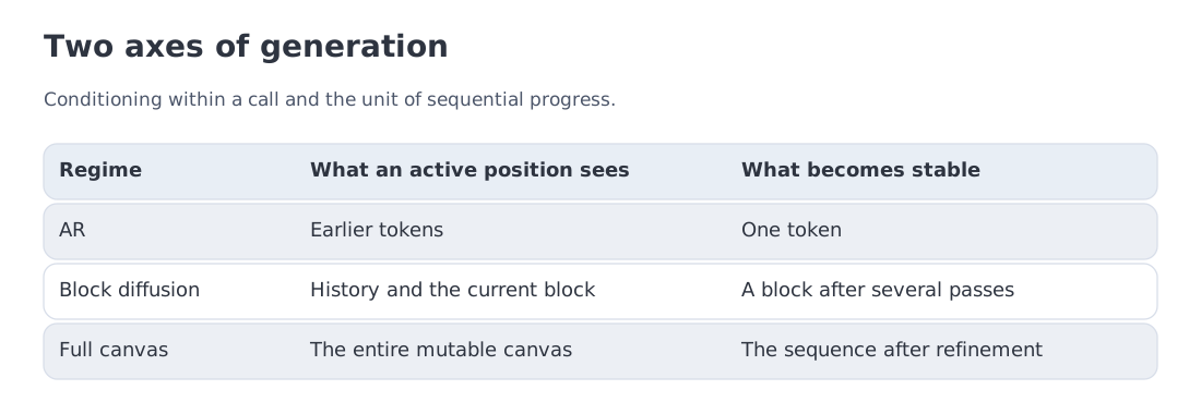 Two independent design axes: causal versus bidirectional conditioning, and token versus block versus canvas as the unit of sequential progress.
4. A two-axis map
It helps to ask two questions separately:
- Which positions may condition one another inside a network call?
- How much of the output becomes stable before the next call?
| Regime | Stable state before a call | Positions updated by a call | Cache implication |
|---|---|---|---|
| AR | causal prefix | one new token | exact prefix KV cache |
| full masked diffusion | fixed condition plus mutable canvas | many canvas positions | mutable canvas is recomputed |
| block diffusion | completed blocks | one current block | completed prefix is cacheable |
| token editing | a partially stable draft | selected replacements | depends on which regions remain stable |
| flexible masked diffusion | current variable-length draft | unmasking and/or insertion | method-specific |
A call can refine positions in the current block without completing that block. Several calls may be needed before its tokens become stable. The map prevents two common errors. A diffusion model is not necessarily restricted to a fixed final length. Conversely, block diffusion does not become ordinary AR merely because blocks are ordered causally: the active block is still modeled with bidirectional, any-order refinement.
5. The absorbing-mask forward process
The main formalism in this module is absorbing masked diffusion. It is a particular discrete kernel, not a definition of all diffusion language models. D3PM also permits random substitutions and more general transition matrices.
Let be a clean sequence. Under a linear schedule, each eligible position is retained with probability and replaced by a special mask state with probability :
The symbol is 1 for and 0 otherwise. This equation specifies a marginal at a single time. A monotone sample path can be constructed by drawing one threshold per position and masking that position whenever . Resampling fresh Bernoulli variables at every time gives the right marginals but does not trace one absorbing path.
“Absorbing” describes the forward chain: after entering the mask state, the position does not spontaneously return to content. The learned reverse model predicts clean tokens from the partially observed sequence.
For conditional generation, a prompt can be marked ineligible for corruption. Only the answer region follows the mask process. This separation becomes important in systems such as DiffusionGemma, where the prompt is encoded and cached while the generation canvas is repeatedly recomputed.
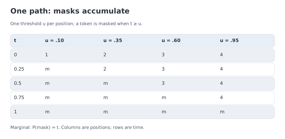 Absorbing masking is the chapter’s reference kernel. Other discrete diffusion models may use substitution noise or a general transition matrix.
6. Worked example A: a mask schedule
With eight positions and four model calls, use the target counts
One explicit schedule is
Exactly two positions become stable after each call. When , duplicate counts can appear; a model call may then perform work without revealing a new token.
Here is a discrete iteration index, whereas in the forward process is a continuous corruption time. The count schedule tells us how many positions to reveal; we still need an objective that teaches the network what to put there.
7. Training objective and likelihood
Training requires an objective before it requires a reveal policy. Ideally we would maximize the probability of a clean sequence, summing over all hidden paths that could have produced it. That sum is generally difficult. An evidence lower bound (ELBO) provides a tractable lower bound on log probability; its negative, NELBO, is an upper bound on negative log-likelihood.
For a linear absorbing-mask process, a clean-token parameterization that copies observed tokens and excludes mask from clean predictions simplifies the continuous-time objective. One sampled slice contributes:
Here denotes the masked positions, and natural logarithms give the loss in nats. Averaging the slice over uniform time and the corruption process gives
The bound applies to this complete objective, not to every sampled slice individually. With retention probability , the general weighting becomes . Low-noise slices hide fewer positions, so a hidden position receives greater weight.
For a continuous linear masking process, the slice weight is . At , the values are , , and . Early-time slices contain fewer corrupted positions, so each receives greater weight. This may increase estimator variance and motivates alternative schedules or time-sampling strategies in practical training.
Reduction is part of the objective. Dividing by a fixed sequence length changes a constant scale. Dividing by the random mask count changes the relative weight of examples and requires a correction if the same estimator is intended. A corruption sample with no masks contributes zero to the sum. Discarding it, or forcing one position to be masked, changes the sampling law.
Suppose four masked target tokens receive probabilities
at . Then
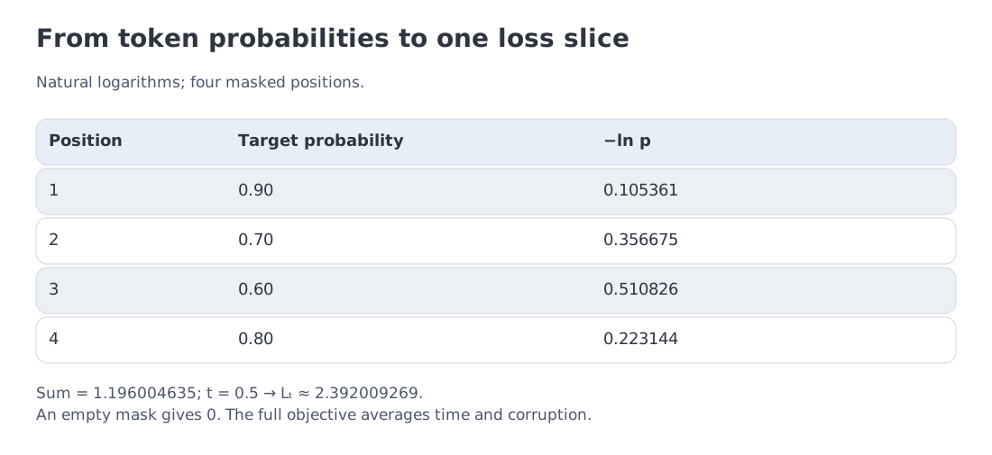 The loss contract: masked positions, time weighting, and an explicit reduction convention. Likelihood interpretation depends on the forward process and estimator.
The value has zero measure under a continuous sampler but remains a software edge case because is undefined.
Likelihood language also needs care. AR provides a direct left-to-right NLL — Negative Log-Likelihood. Many diffusion models optimize an ELBO — Evidence Lower Bound or report NELBO — Negative Evidence Lower Bound. Yet masked diffusion can be designed as a likelihood-oriented language model, as MDLM demonstrates. A fair comparison records the estimator, time discretization, and number of Monte Carlo samples instead of treating every reported “perplexity” as the same object.
8. Any-order training and its limits
Random corruption turns one document into many conditional prediction tasks. A person’s name may be observed while the relation is hidden in one sample, and the reverse may occur in another. This offers a more symmetric training signal than a single left-to-right order.
For a uniform-order objective, masked diffusion can be related to autoregressive factorizations averaged over permutations. The Any-Order GPT study also finds that many orders are less informative than natural left-to-right structure. The result is a design trade-off, not a contradiction: order diversity is useful, but language still has asymmetric sequential regularities.
The same caution applies to the reversal curse. Consider the fictional fact “Anna Vetrova wrote The Quiet Harbour.” A model may complete the author’s name with the book title yet fail to name the author when asked who wrote that book. Reversing the question is not the same as claiming that authorship is a symmetric relation. LLaDA reported a striking reversal-poem result. Later work, DiffER, found that dLLMs can still fail reversed relations because of fragmented entities, asymmetric training data, or entirely missing reverse facts. Bidirectional conditioning removes one architectural asymmetry; it does not invent absent evidence.
A related empirical result appears in data-constrained training. When a finite corpus is reused for many epochs, masked diffusion exposes the model to varied conditional tasks. Diffusion Beats Autoregressive in Data-Constrained Settings reports an advantage under the studied data/compute regimes. The claim should remain local to those regimes rather than becoming a universal statement about data efficiency.
9. Sampling and worked example B
A denoising network returns token distributions, while a sampler defines how to use them. For the linear absorbing process, one standard reverse transition from time to leaves a masked position masked with probability and reveals it with probability , using the predicted clean-token distribution. Visible positions are copied. This connects the forward kernel to a reverse transition; deployed policies often alter the schedule or position choices to trade quality for speed.
Our teaching trace uses a fixed mask-count schedule and greedy token choices. It makes the operations inspectable but does not establish exact sampling from the data distribution. Confidence-based reveal has no universal distribution-correction guarantee analogous to the speculative algorithm in Module 11.
A generic iteration performs five operations:
- optionally remask open positions using scores saved from earlier predictions;
- call the model once on that actual corrupted canvas;
- choose candidates and rank masked positions;
- reveal enough positions to meet the next mask count;
- save the result and confidence scores for the next iteration.
Possible ordering rules include random reveal, maximum candidate probability, minimum entropy, a learned policy, block-specific schedules, and task-dependent heuristics.
Candidate confidence is the single probability , whereas entropy measures uncertainty across the whole positional distribution. Low entropy means that probability is concentrated among fewer alternatives. The rankings can differ, especially when a candidate is sampled rather than chosen by argmax.
The first frozen trace uses fixed logits and opens two positions per step. Six of eight final tokens match the targets, regardless of the order in which all greedy candidates are eventually revealed. It tests scheduling, not context sensitivity. A second notebook experiment makes predictions depend on previously revealed anchors; there the order can change the final answer.
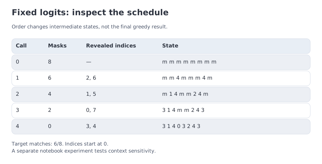 One call per iteration, candidate tokens for every position, a confidence ranking, and an exact target mask count.
A two-token example explains why extra passes can matter. Suppose the source emits only or , each with probability . With both positions masked, each marginal assigns to A and B. Sampling them independently in one pass produces with probability each; half the outputs violate the source's dependency. Reveal one token and recompute the other conditional, and the dependency can be recovered. Parallel predictions may be individually well calibrated while their product is a poor joint model.
Remasking can revisit a poor early choice after more context becomes available. Revision spends extra calls or reduces net progress at a fixed call budget. In our implementation, selected positions are masked before the network is invoked; logits computed while a token was still visible are not treated as predictions from a masked input. The useful metric is therefore not “tokens predicted per pass” alone; it is final committed output per pass at a target quality.
DiffusionGemma illustrates a more sophisticated policy. Its recommended EB — Entropy Bound sampler selects low-entropy positions subject to a bound on dependence between jointly revealed positions (a mutual-information bound), renoises unselected positions, and stops only when entropy and prediction stability criteria are satisfied. The sampler is part of the released system contract, not an interchangeable afterthought.
10. A generic roofline calculation
Return to the hypothetical dense 8B model. Nothing in this section describes DiffusionGemma’s MoE traffic.
For a 1024-position canvas, one ideal pass performs
At 990 TFLOP/s, the compute floor is
which is larger than the 4.776-ms weight-stream floor. For calls,
| Calls | Arithmetic ceiling |
|---|---|
| 16 | 3867.2 tok/s |
| 64 | 966.8 tok/s |
| 128 | 483.4 tok/s |
The continuous parity point with the batch-one AR ceiling is approximately . Integer call counts give 295 as the largest value still above that ceiling.
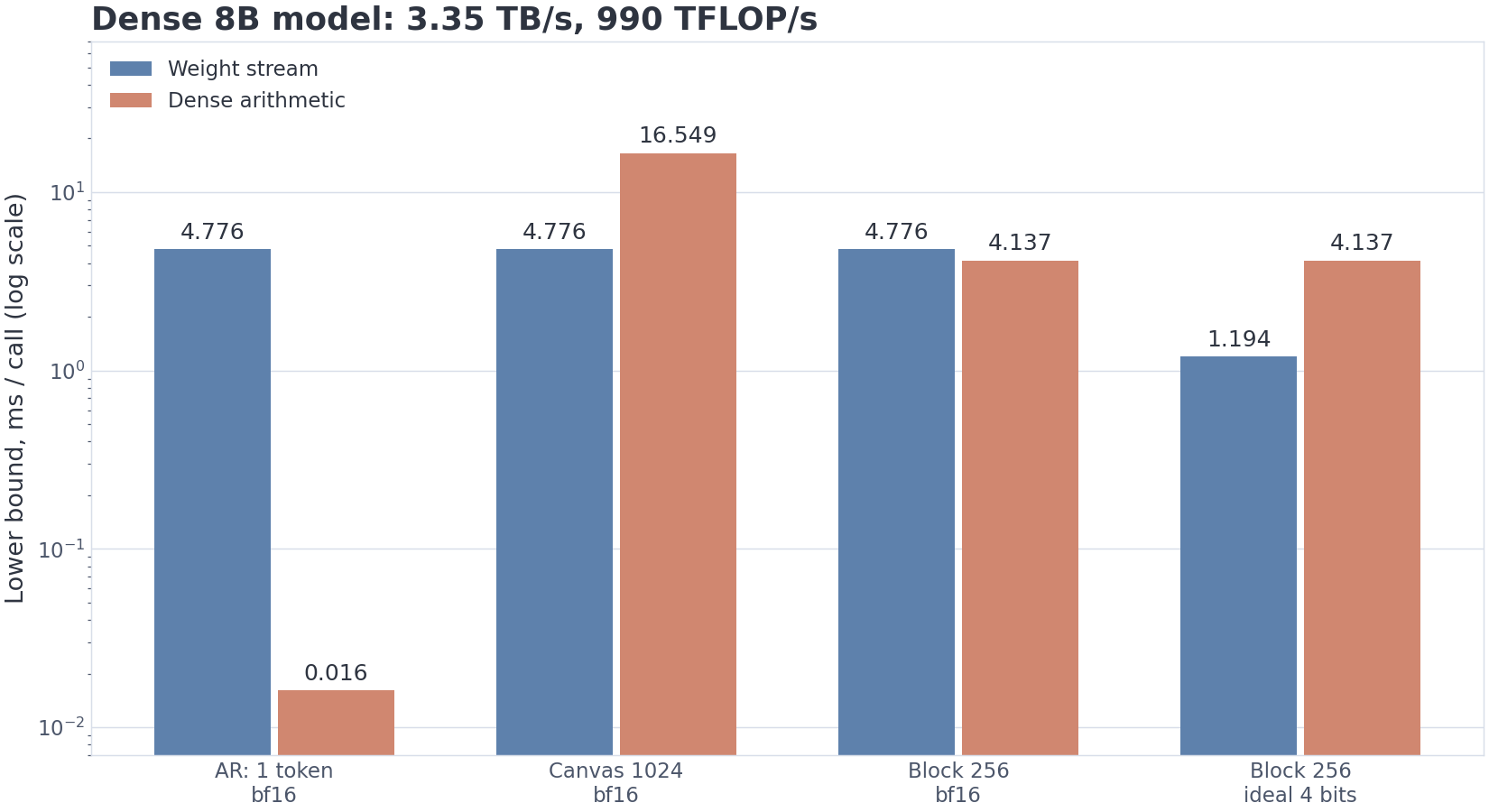 Generic dense-8B roofline. The 0.338% figure is ideal compute time divided by the simplified step floor, not measured accelerator utilization.
The calculation is useful precisely because it is narrow. It excludes attention’s sequence-length cost, KV traffic, activations, communication, routing, batching, kernel overhead, and actual utilization.
11. Steps, batching, and weight precision
Autoregressive batching also amortizes weight reads. Under a crude linear batch-throughput approximation, the diffusion ceiling equals AR at
This is not a claim that the fifth concurrent request always erases the benefit. Actual batching changes KV traffic, tensor shapes, occupancy, and latency objectives. The calculation identifies the direction: low-batch interactive use is the most favorable regime for parallel denoising.
The same dense model gives a second teaching comparison at a 256-token block. The compute floor is 4.137 ms. With 16 GB of bf16 weights, the 4.776-ms memory floor still dominates. If every parameter were ideally stored in four bits, the payload would be 4 GB and the memory floor 1.194 ms; the block would become compute-bound. At 16 calls, the arithmetic ceiling is again 3867.2 tok/s.
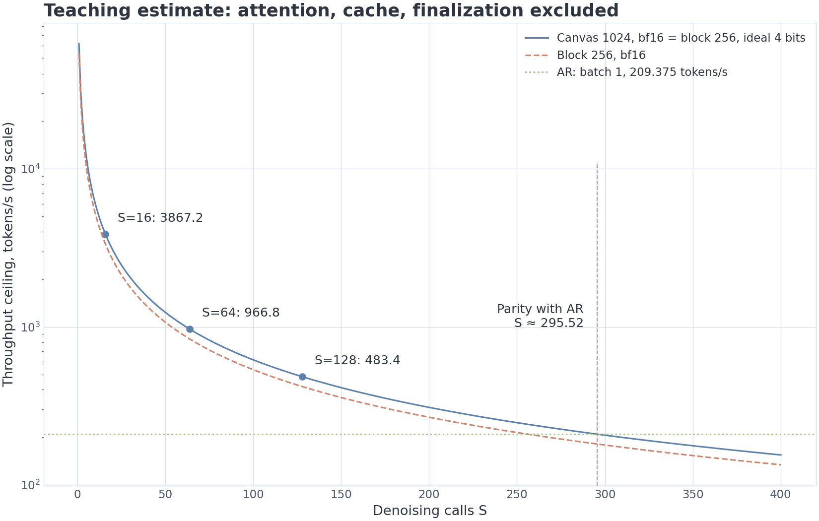 Throughput versus call count for the generic dense-8B scenario. The four-bit line is an arithmetic payload hypothesis, not a DiffusionGemma checkpoint measurement.
A sparse MoE invalidates a naive substitution of “active parameters” for bytes per call. Different canvas positions can select different experts, so the union of touched expert weights may be much larger than a single token’s active count. This is the key reason to keep the following released-model passport separate.
12. Level-1 code
The minimal implementation must make two contracts visible: the loss only includes corrupted positions, and one sampler iteration makes exactly one network call before revealing the scheduled number of tokens.
"""M12: summed masked loss and deterministic reveal schedule."""
import numpy as np

def linear_mask_schedule(length: int, steps: int) -> tuple[int, ...]:
    """Target counts from fully masked to fully revealed."""
    if any(isinstance(v, (bool, np.bool_)) or
           not isinstance(v, (int, np.integer)) or v <= 0
           for v in (length, steps)):
        raise ValueError("length and steps must be positive")
    return tuple(
        (int(length) * remaining + int(steps) - 1) // int(steps)
        for remaining in range(steps, -1, -1)
    )

def dllm_loss(logits, target_ids, loss_mask, time: float) -> float:
    """(1/t) times the summed NLL on explicitly masked positions."""
    logits = np.asarray(logits, dtype=np.float64)
    target_ids = np.asarray(target_ids)
    loss_mask = np.asarray(loss_mask)
    if logits.ndim != 2 or target_ids.shape != (logits.shape[0],):
        raise ValueError("expected logits [T,V] and target_ids [T]")
    if logits.shape[1] == 0 or target_ids.dtype.kind not in "iu":
        raise ValueError("target_ids must be integers and vocabulary non-empty")
    if np.any(target_ids < 0) or np.any(target_ids >= logits.shape[1]):
        raise ValueError("target IDs must be in [0, V)")
    if loss_mask.shape != target_ids.shape or loss_mask.dtype.kind != "b":
        raise ValueError("loss_mask must be boolean [T]")
    if isinstance(time, (bool, np.bool_)) or not (0.0 < time <= 1.0):
        raise ValueError("time must be in (0,1]")
    if not np.isfinite(logits).all():
        raise ValueError("logits must be finite")
    shifted = logits - logits.max(axis=-1, keepdims=True)
    log_probs = shifted - np.log(np.exp(shifted).sum(axis=-1, keepdims=True))
    nll = -log_probs[np.arange(target_ids.size), target_ids]
    return float(nll[loss_mask].sum() / time)

def sample_dllm(predict, length: int, steps: int, mask_id: int):
    """Greedy confidence reveal with one model invocation per iteration."""
    schedule = linear_mask_schedule(length, steps)
    if isinstance(mask_id, (bool, np.bool_)) or not isinstance(mask_id, (int, np.integer)):
        raise ValueError("mask_id must be an integer")
    vocabulary = None
    tokens = np.full(length, mask_id, dtype=np.int64)
    trace = []
    for step, target_masked in enumerate(schedule[1:], start=1):
        logits = np.asarray(predict(tokens.copy(), step), dtype=np.float64)
        if logits.ndim != 2 or logits.shape[0] != length or logits.shape[1] == 0 or not np.isfinite(logits).all():
            raise ValueError("predict must return finite logits [T,V]")
        if vocabulary is not None and logits.shape[1] != vocabulary:
            raise ValueError("predict changed vocabulary size")
        vocabulary = logits.shape[1]
        if 0 <= mask_id < vocabulary:
            raise ValueError("mask_id must lie outside the vocabulary")
        shifted = logits - logits.max(axis=-1, keepdims=True)
        probs = np.exp(shifted)
        probs /= probs.sum(axis=-1, keepdims=True)
        candidates = probs.argmax(axis=-1)
        confidence = probs[np.arange(length), candidates]
        masked = np.flatnonzero(tokens == mask_id)
        open_count = masked.size - target_masked
        order = np.lexsort((masked, -confidence[masked]))
        opened = masked[order[:open_count]]
        tokens[opened] = candidates[opened]
        trace.append((tuple(opened), tokens.copy()))
    return tokens, trace
Read the loop as an execution record: one copied input goes into the network, the stored output supplies both candidates and scores, and only then does the state change. Equal scores choose the lower position index. A schedule with more calls than tokens may include calls that reveal nothing.
Using −1 outside the output vocabulary is a teaching interface, not a universal model requirement. Real models often include a special mask token in their vocabulary and exclude it from final clean-token predictions through parameterization or filtering. The notebook adds categorical draws, entropy ranking, and remasking. Adaptive production samplers need not follow our fixed mask counts.
14. Block diffusion, length, and caching
A mutable bidirectional canvas cannot use an ordinary causal KV cache internally: changing one position can change representations at every other position on the next call.
Block diffusion separates completed history from a mutable block of length . Cache validity requires the history's states to be independent of future blocks. It does not require token-wise causal attention within every completed block: bidirectional attention inside an already completed block is compatible with block causality. Section 19 uses the simpler special case of a token-causal prefix.
The active block reads that history and all of its own positions. After final token choices, the cache must represent the clean block. The last denoising call may have seen masks or earlier values, so its K/V cannot automatically serve as the completed history. BD3-LM runs the clean block to obtain cache states; DiffusionGemma uses its encoder for this step. That pass and prompt processing contribute to end-to-end latency, though they are omitted from the narrow arithmetic in Sections 10–11.
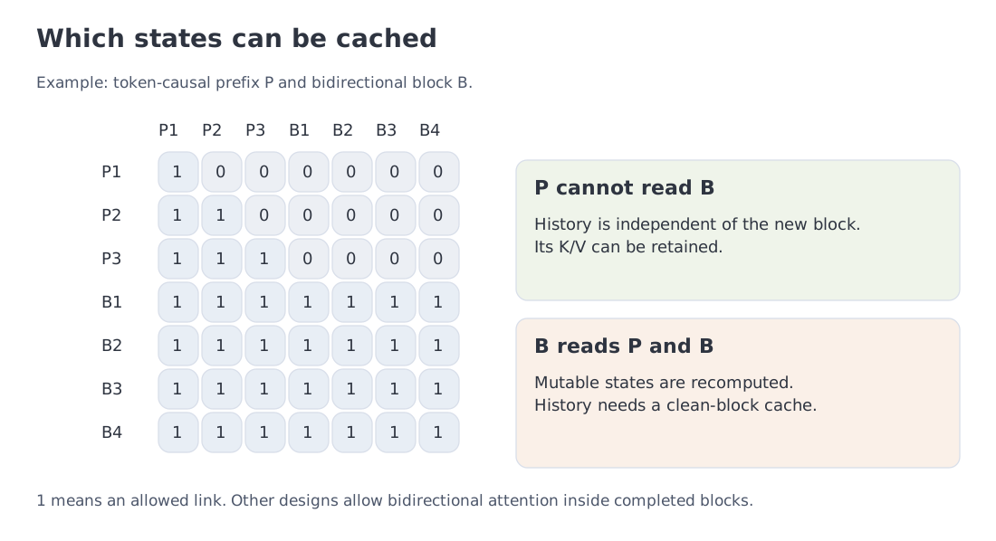 The teaching attention mask makes the completed prefix independent of the active block. Cache states must correspond to the finalized history.
As changes:
- approaches AR;
- larger blocks expose more parallel work;
- completed blocks become cacheable;
- the active block remains bidirectional;
- output length can grow block by block.
BD3-LM formalizes this class. MDLM also presents semi-autoregressive variable-length sampling, FlexMDM inserts mask states, and iLLaDA reports variable-length generation. Block diffusion is therefore one strong design, not a monopoly on flexible length.
LLaDA2.0 uses block size as a conversion curriculum. During warmup:
The stable phase trains full-sequence masked diffusion; decay returns to smaller blocks for efficient inference. LLaDA2.1 adds Token-to-Token editing so a revealed value may later be replaced. The published mechanism revises values while keeping the current positions.
15. Reading the DiffusionGemma passport
DiffusionGemma is a useful case because its model card exposes architecture, sampler, and hardware conditions rather than only a headline TPS number.
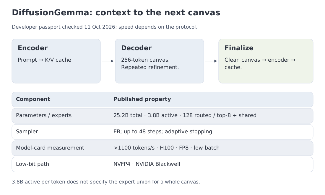 An autoregressive prompt encoder, cacheable context, a bidirectional diffusion canvas, sparse MoE routing, and separate H100 FP8 and Blackwell NVFP4 paths.
| Field | Released contract |
|---|---|
| architecture | encoder–decoder, block-autoregressive multi-canvas diffusion |
| total / active parameters | 25.2B / 3.8B |
| layers | 30 |
| experts | 128 routed, top-8, plus one shared |
| canvas | 256 tokens |
| context | up to 256K |
| sliding window | 1024 |
| input | text, images, and video represented as frames |
| output | text |
| sampler | Entropy-Bounded Denoising, adaptive stopping, at most 48 calls |
| committed progress | typically 15–20 final tokens per forward pass |
| reported speed | over 1100 tok/s, H100, FP8, low batch |
| native low-bit path | NVFP4 on NVIDIA Blackwell |
The prompt is processed by an autoregressive encoder and stored as cacheable context. A bidirectional decoder denoises the active canvas through cross-attention to the prefix. After completion, the canvas is encoded and appended to the prefix cache.
Two idealized four-bit payloads are easy to compute:
Neither is measured bytes per diffusion call. The full bank includes heterogeneous tensors; a 256-position canvas can route tokens to different experts; actual traffic depends on the expert union, precision, metadata, caches, and kernels.
The joint vLLM release report gives 1008 tokens/s on H100 FP8 in its own experiment. That is a separate protocol record from the model card’s “over 1100,” not a number to average into it.
The quality side matters as much as speed. The model card reports lower scores than AR Gemma 4 on many benchmarks, with some exceptions. DiffusionGemma is therefore a point on a quality–latency curve, not proof that a generation paradigm dominates every task.
16. The dLLM landscape on 11 October 2026
The following rows deliberately include the measurement context. Tokens per second without hardware, sampler, and overhead is not a comparable metric.
| System | Access and branch | Published signal | Evidence boundary |
|---|---|---|---|
| LLaDA 8B | open weights, from scratch | 2.3T pretraining tokens | scale result; reversal result belongs to one task |
| LLaDA-MoE 7B-A1B | open weights | sparse diffusion MoE, 1.4B active | active count does not determine runtime speed |
| LLaDA2.0 16B / 100B | open weights, AR conversion | WSD and block diffusion | throughput depends on CAP/dInfer, threshold, and hardware |
| LLaDA2.1 | open weights | Token-to-Token editing | value revision, not insertion-based length editing |
| iLLaDA 8B | open weights, from scratch | 12T pretraining tokens, variable length | foundation-model result rather than a universal TPS claim |
| Mercury 2 | commercial API | 1009 tok/s on Blackwell, 128K | developer-reported product configuration |
| Gemini Diffusion | experimental demo | 1479 tok/s sampling, 0.84 s overhead excluded | sampling rate is not end-to-end latency |
| Seed Diffusion Preview | experimental, code-focused | 2146 tok/s on H20 | developer result on coding workloads |
| DiffusionGemma | open weights | >1100 tok/s, H100 FP8; 15–20 committed tokens/pass | detailed open passport with stated measurement conditions |
Mercury 2 adds reasoning controls, tool use, and schema-constrained JSON to a commercial dLLM API. Gemini Diffusion makes the measurement boundary unusually explicit: 1479 tok/s excludes 0.84 seconds of fixed overhead. Seed Diffusion targets code and reports H20 throughput. None of those numbers can be ranked fairly without rerunning a shared workload.
iLLaDA highlights a different frontier: improving a from-scratch bidirectional model rather than solely accelerating a converted checkpoint. Its 12T-token pretraining run and variable-length generation show that the research space includes foundation-model quality, not only sampler speed.
17. Multimodal diffusion systems
“Multimodal diffusion” can refer to different components.
LLaDA-V applies diffusion language modeling to vision-language understanding: a visual representation conditions a diffusion-generated text response.
LLaDA2.0-Uni discretizes visual inputs through SigLIP-VQ, uses a MoE dLLM backbone over semantic tokens, and employs a separate diffusion decoder to reconstruct images. Text-token diffusion and pixel/latent generation are distinct parts of the stack.
DiffusionGemma accepts interleaved text, images, and video frames but produces text. Its vision encoder does not imply that the response is generated by the same image diffusion decoder used in a text-to-image system.
The useful passport question is:
Which object is diffused—language tokens, visual semantic tokens, a continuous image latent, or several of these at different stages?
Without that distinction, two systems bearing the same label may have entirely different compute and memory profiles.
20. Takeaways and sources
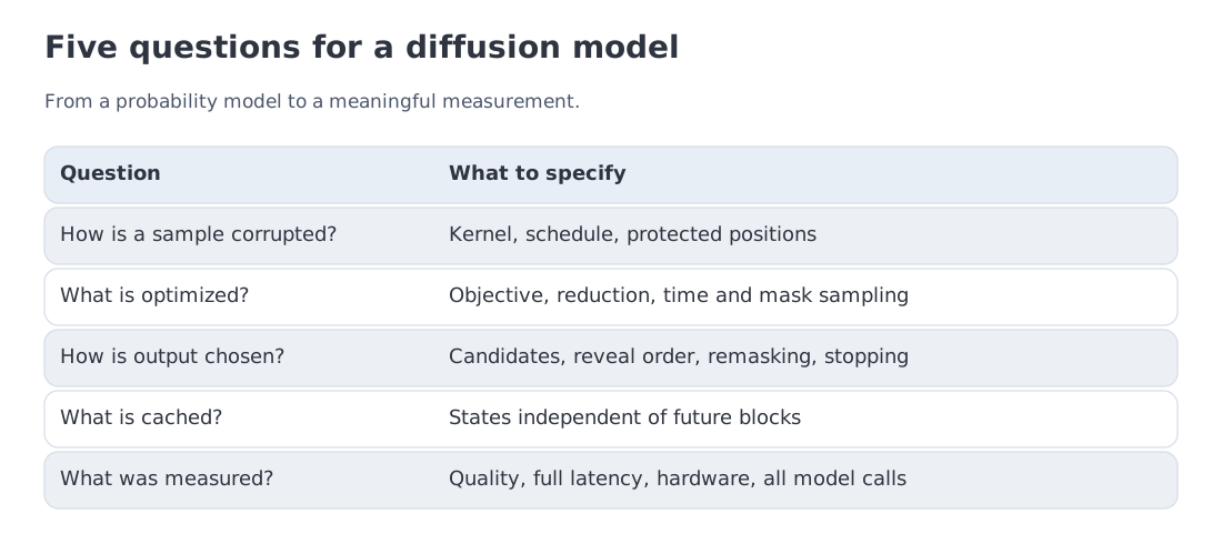 The forward kernel, loss, sampler, teaching roofline, block spectrum, and a released-system evidence passport on one page.
Generation protocol. AR commits one token. Masked diffusion revises a canvas. Block diffusion makes completed history independent of future blocks and cacheable.
Forward process. The chapter uses an absorbing mask; discrete diffusion supports other kernels.
Objective. The 2.392009269 example uses time weighting and sum reduction over corrupted positions. Likelihood claims require an explicit estimator.
Sampling. Reveal order, remasking, entropy bounds, and adaptive stopping are part of the algorithm, not cosmetic decoding flags.
Roofline. The 8B/H100 figures are a generic teaching floor. The 0.338% quantity is not measured utilization.
DiffusionGemma. 25.2B total / 3.8B active, 128 routed experts with top-8 plus one shared, 256-token canvas, 15–20 committed tokens per pass, over 1100 tok/s on H100 FP8, and a native NVFP4 Blackwell path. Four-bit parameter arithmetic does not equal measured per-pass traffic.
Evidence. Mercury, Gemini, Seed, and DiffusionGemma report throughput under different protocols. Always keep hardware, precision, sampler, batch, overhead, and quality attached.
Primary sources
- D3PM
- Diffusion-LM
- SEDD
- FlexMDM
- DiffusionGemma in vLLM
- MDLM
- LLaDA
- BD3-LM
- Any-Order GPT as Masked Diffusion
- Data-Constrained Diffusion
- LLaDA2.0
- DiffER
- LLaDA2.1
- LLaDA2.0-Uni
- iLLaDA
- DiffusionGemma model card
- DiffusionGemma announcement
- Mercury 2
- Gemini Diffusion
- Seed Diffusion
Next: Module 13 returns to the autoregressive path for supervised fine-tuning: preparing demonstrations and teaching a pretrained model the response patterns expected of an assistant.
Landscape verified: 11 October 2026. Product throughput figures are developer-reported results under different hardware and sampling protocols. Sections 10–11 describe a separate generic dense-8B teaching scenario.