Module 17. Embeddings, Retrieval, and RAG
“Modern LLMs” course · Module 17 lecture · edition 2026.10.25
What this module is about. A language model cannot keep every private document, recent policy update, source citation, and access rule inside its parameters. Retrieval-Augmented Generation, or RAG, gives the model an external evidence path. Yet RAG is not one search call followed by one prompt. A query moves through a sequence of compressions: documents become chunks, chunks become representations, an index keeps only a candidate set, a reranker keeps an even smaller set, and a context builder decides which evidence reaches the generator. Each compression saves time or memory, and each can discard the answer. We will use one query as the thread through the module and ask four questions at every stage: what information is retained, what is lost, how the stage is measured, and what the next stage can still repair.
Prerequisites. Module 2 develops tokenization and embeddings; Module 10 provides the prefill/decode cost model; Module 13 provides the data-engineering discipline used for examples and evaluation. All retrieval definitions, formulas, and numerical scenarios are developed here, so the lecture remains self-contained.
Reading routes
First reading: follow Sections 1, 4–5, 7, 10–12, and 15–17, then the conclusion. Keep asking which stage can discard the evidence. Section 10 defines the three metrics before presenting results, so the index internals can wait.
Second reading: add the history in 2–3, storage and search arithmetic in 6 and 8, index design in 9, and implementation in 13–14. Work through 18–19. Trace one saved query through every ranking, predict what a smaller context budget will remove, and then run the change.
Reference reading: return to the resource tables, the embedder passport in 17, metric equations, and primary sources. Timing numbers describe a specified scenario and must be replaced by measurements when choosing a deployed system.
1. Motivation: one query, four opportunities to lose the answer
Suppose a user asks a precise question about a large internal corpus. The relevant passage exists, but the generator cannot read every document on every request. A retrieval system therefore compresses the corpus repeatedly.
The first compression is chunking. A long document is divided into retrievable units. If the boundary falls between a definition and the sentence that uses it, neither chunk may be sufficient.
The second compression is representation. A sparse index keeps terms and their frequencies; a dense encoder maps a passage into a vector; a late-interaction system keeps several token vectors. Each representation preserves different evidence and discards different detail.
The third compression is candidate search. Exact search compares the query with every stored representation. Approximate nearest-neighbor search inspects only part of the index, gaining speed at the risk of missing a relevant item.
The fourth compression is context assembly. Even a good candidate list cannot be sent to the model without limits. The system removes duplicates, applies permissions, chooses an order, and fits the selected passages into a token budget.
The generator sees only what survives all four stages. If the answer is wrong, “the RAG system failed” is not yet a diagnosis. The chunk may never have contained the evidence; the representation may have hidden it; approximate nearest-neighbor (ANN) search may have missed it; fusion may have ranked it too low; or the context builder may have dropped it at the budget boundary.
This viewpoint gives the module its central discipline: evaluate every irreversible reduction at the point where it occurs. Retrieval quality is not a property of the embedding model alone, and answer quality is not a sufficient diagnostic for retrieval.
2. Historical progression: each generation restored a signal that the previous one had compressed away
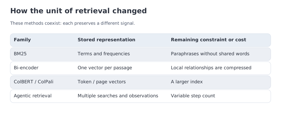 From inverted indexes to dense retrieval, late interaction, multimodal retrieval, and agentic search. Each step restores a kind of evidence that an earlier representation made difficult to recover.
The earliest large-scale search systems relied on inverted indexes. TF-IDF (Term Frequency–Inverse Document Frequency) and BM25 (Best Matching 25, the historical name of the ranking function) answered a concrete question efficiently: which documents contain these terms, and how unusual are those terms in the collection? BM25 refined this branch by balancing term frequency, document length, and corpus rarity. For identifiers, names, error codes, and exact phrases, that literal signal remains difficult to replace.
Dense retrieval changed the unit of comparison. DPR (Dense Passage Retrieval) and related bi-encoders learned separate functions for queries and passages, turning semantic similarity into geometry. A question and a relevant paragraph no longer needed to share the same wording. The gain came with a new loss: one vector had to summarize an entire passage before the query ever arrived.
ColBERT (Contextualized Late Interaction over BERT) and other late-interaction systems recovered part of that token-level structure. Documents could still be encoded in advance, but matching happened between sets of token vectors rather than between two single points. The index became larger, yet the scorer could preserve local alignments that a single-vector representation had collapsed.
The next wave addressed the documents themselves. Late chunking retained long-document context before pooling into chunks. ColPali treated rendered pages as visual objects instead of forcing every table, layout cue, and figure through OCR. Qwen3 Embedding combined multilingual embedding and reranking checkpoints in several sizes. Benchmarking IR (BEIR), the Massive Text Embedding Benchmark (MTEB), and the Massive Multilingual Text Embedding Benchmark (MMTEB) broadened evaluation beyond one English retrieval collection.
The original RAG formulation by Lewis et al. treated the retrieved document as a latent variable. It combined generation probabilities across documents, weighted by retrieval probabilities: RAG-Sequence used one latent document for a whole output, while RAG-Token marginalized separately at each position. The application pipeline studied here instead assembles retrieved passages into a shared generator context. These are different ways to connect retrieval and generation.
Subsequent RAG research also moved beyond a fixed retrieval pass. Hypothetical Document Embeddings (HyDE) changed the query representation, Self-Reflective Retrieval-Augmented Generation (Self-RAG) learned when to retrieve and critique evidence, Recursive Abstractive Processing for Tree-Organized Retrieval (RAPTOR) introduced hierarchical summaries, and GraphRAG targeted corpus-level questions through graph and community summaries. The final transition is architectural: retrieval becomes a tool in an agent loop. The model can search, inspect evidence, reformulate, and decide whether another retrieval step is worth its cost.
The historical pattern is therefore not “lexical search was replaced by vectors.” It is a sequence of trade-offs. Each method makes one form of evidence cheap enough to search, then later methods recover detail that the compression had hidden.
3. A bridge to classical methods: three old problems inside RAG
Information retrieval: relevance under incomplete evidence
BM25, relevance judgments, Mean Reciprocal Rank (MRR), Recall, and normalized Discounted Cumulative Gain (nDCG) come from information retrieval, not from generative AI. That tradition already distinguished between finding a relevant item and ordering several relevant items well. RAG inherits the same distinction, with one additional downstream consumer: a language model that may ignore, misread, or overstate retrieved evidence.
Metric learning: place useful pairs close and confusing pairs apart
Dense retrieval is a form of metric learning. A query encoder and a document encoder produce vectors, and training makes a relevant pair score higher than negative pairs. The loss says little unless we also ask where the negatives came from. Random negatives rapidly become trivial. Hard negatives define the decision boundary but may accidentally be relevant, creating false-negative gradients.
Cascades and selective computation
A search cascade resembles a classical detection pipeline. A cheap stage aims for high recall and allows many false positives. A more expensive stage spends computation only on the reduced candidate set. The correct optimization target is not “make every stage individually perfect.” It is to preserve enough recall early that later stages can recover precision without exceeding latency and memory budgets.
These ancestors suggest a useful reading rule. Sparse retrieval, dense retrieval, ANN, reranking, and generation are not competing products. They are stages with different jobs, different failure costs, and different evaluation metrics.
4. BM25 and learned sparse retrieval: the branch that protects exact terms
An inverted index maps each term to the documents containing it, together with occurrence information needed for scoring. A lexical retriever uses these lists to find candidates. Each document is represented by vocabulary coordinates rather than a single dense vector. The classic BM25 score for query and document can be written as
Here denotes the query, the document, and a tokenized term. The frequency counts occurrences of in . Document length and collection mean use that same tokenizer.
The parameter controls frequency saturation; controls length normalization. With , length has no effect; with , the normalization uses the full length ratio. Values such as and are starting points to evaluate on the target collection.
Our implementation chooses the positive IDF convention
counts documents; counts documents containing the term. With 100 documents, a term found in one has weight , whereas one found in fifty has weight . Repeating a query term repeats its contribution in this implementation; other query-frequency conventions need not match it.
Literal retrieval is only as literal as its analyzer. The notebook's word tokenizer splits TS-999 into ts and 999, and 4.7.3 into three numbers. If the entire identifier matters, inspect the analyzed representation and preserve an exact field where needed. BM25's name alone promises no such preservation.
The three components have different roles.
- rewards terms that are rare in the collection.
- The fraction involving saturates repeated occurrences; the tenth repetition should not be worth ten times the first.
- The length normalization prevents long documents from winning merely because they contain more words.
BM25 is especially strong when relevance is anchored by a literal string: a product code, stack-trace fragment, legal clause number, API name, or person. A dense encoder may place several related identifiers near one another, while a lexical index retains the distinctions represented by its analyzer.
Learned sparse methods such as SPLADE (Sparse Lexical and Expansion Model) keep the inverted-index execution model but learn term weights and expansion terms. A passage about “heart attack” may activate a “myocardial” dimension even when that word is absent. The representation is still sparse enough for posting-list retrieval, yet it acquires some semantic generalization.
This branch has its own failure mode. Literal terms may be absent from a paraphrased query; vocabulary expansion may introduce noisy associations; and exact matching cannot by itself decide whether the same term is used in the relevant sense. The dense branch is introduced not because sparse retrieval is obsolete, but because the two branches lose different information.
5. Dense bi-encoders: learning a semantic space
In Module 2, an embedding was a table row selected by one token ID. Retrieval needs a representation of an entire query or passage. A Transformer encoder first contextualizes the tokens, then combines their states into one vector, for example by averaging or using a designated position. This pooling rule must match the model’s training. An arbitrary row of an LLM’s input table is therefore not a substitute for a retrieval representation.
A bi-encoder computes a query vector and a document vector independently. Similarity is then a cheap function such as a dot product or cosine:
The decisive engineering advantage is precomputation. Document vectors are built once and stored in an index. At request time the system encodes only the query and searches the stored geometry.
A common contrastive objective places the positive document above negatives in the same batch:
The temperature controls sharpness: reducing it emphasizes the largest scores, including incorrectly preferred negatives. It cannot repair a mislabeled pair.
The denominator converts other documents in the batch into negatives. This makes large batches attractive, but it also creates a data-quality question: another query's positive document may be relevant to as well. Treating it as negative produces a false-negative signal.
Hard negatives are usually more informative. A lexical or earlier dense retriever finds passages that look plausible but are not judged relevant. They force the model to separate near misses—two similar policies, two software versions, or two entities with related names. Yet hard-negative mining must be audited: the better the retriever, the more likely it is to surface unlabeled positives.
Instruction-aware embedding models add another conditioning channel. A query prefix such as “retrieve passages that answer the question” distinguishes search from clustering or semantic similarity. E5 popularized explicit input prefixes; more recent families expose task instructions or a prompt_name interface. This means the exact text given to the encoder is part of the retrieval contract, not a harmless wrapper.
Pooling is another quiet design choice. A CLS token, mean pooling, last-token pooling, or a learned head can produce different spaces from the same backbone. Before adopting an embedding model, the system should verify the documented pooling rule, normalization, maximum length, and query/document prefixes rather than infer them from the architecture name.
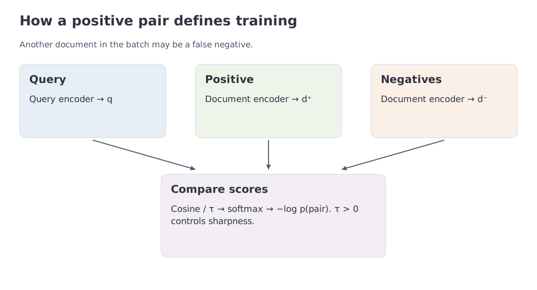 A positive pair, in-batch negatives, hard negatives, and the two-stage training pattern. The quality of the negative set defines the boundary learned by the retriever.
6. Matryoshka Representation Learning (MRL), quantization, and worked example A: the price of storing meaning
A dense index may contain millions or billions of vectors. The storage question is therefore part of model selection.
For vectors of dimension and bytes per coordinate, the raw payload is
Take and .
| Representation | Effective payload | Decimal GB | Binary GiB |
|---|---|---|---|
| fp32 | 32 bits/component | 40.96 | 38.147 |
| fp16 | 16 bits/component | 20.48 | 19.073 |
| int8 | 8 bits/component | 10.24 | 9.537 |
| binary | 1 bit/component | 1.28 | 1.192 |
| MRL prefix 256 + int8 | 256 bytes/vector | 2.56 | 2.384 |
The table counts vectors only. Graph edges, posting lists, centroids, codebooks, document IDs, replicas, and allocator overhead are separate.
Matryoshka Representation Learning (MRL) trains several prefixes of one vector to be useful representations. If the model is trained at dimensions such as 64, 128, 256, 512, and 1024, then the first 256 coordinates can serve as a compact embedding after renormalization. This is not a license to truncate an arbitrary embedding model. The nested property must be part of training and validated for the released checkpoint.
MRL supports a useful cascade. A short prefix performs coarse search over the whole corpus; full vectors rerank only the candidate set. The same checkpoint can therefore trade memory and quality without maintaining several unrelated encoders.
Scalar or binary quantization attacks a different dimension. It reduces the bits per retained coordinate. MRL and quantization can be composed because one shortens the vector and the other compresses each coordinate. The quality cost depends on the embedding distribution and the index, so storage ratios are not retrieval guarantees.
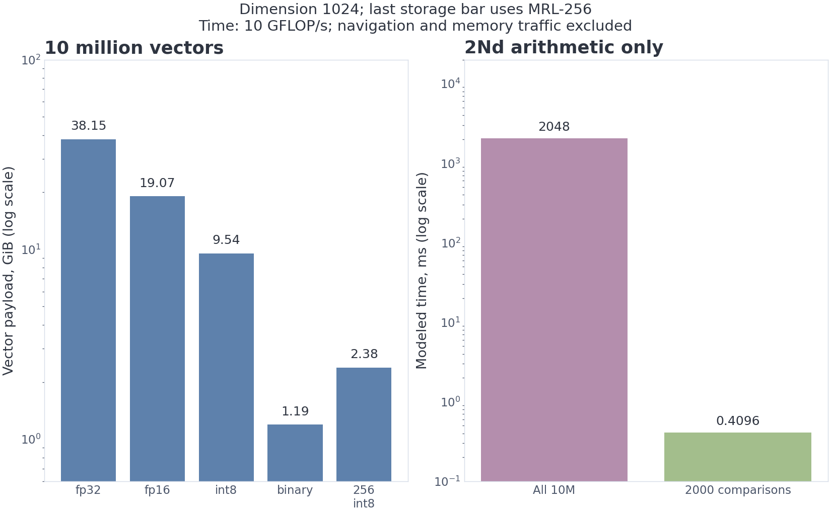 Raw storage for 10M 1024-dimensional vectors and the arithmetic exact-search/shortlist comparison used throughout the module.
7. One vector, one pair, or a matrix: where query-document interaction happens
Retrieval architectures can be arranged by the moment at which the query and document are allowed to interact.
Bi-encoder: interaction after compression
The document is reduced to one vector before the query is known. Search is cheap and scalable, but all token-level structure must survive that compression indirectly.
Cross-encoder: interaction before scoring
A cross-encoder receives the query and document jointly:
[CLS] query [SEP] document [SEP]
Self-attention can compare any query token with any document token, and a head emits one relevance score. Joint encoding can improve ordering on a bounded candidate set, but the outcome still depends on training and the task. The price is that document scores cannot be precomputed: every query-document pair must be jointly encoded. The pairs can be batched; they do not require sequential model calls. Pair count measures work, while batch size and execution determine latency.
Late interaction: interaction after token encoding
ColBERT stores multiple vectors per document. One common MaxSim-style score is
Document token vectors are indexed in advance, while matching remains token-aware. Late interaction therefore occupies a middle point: more expressive than one-vector search and more indexable than a full cross-encoder, but with a substantially larger index.
ColPali applies late interaction to rendered document pages, retaining visual features that OCR and text parsing may discard. Its authors evaluated this approach on ViDoRe, a collection of page-retrieval tasks. Their results do not make text extraction unnecessary: exact strings, copyable content, metadata filtering, and accessibility still benefit from a text path. The visual branch provides another candidate source with its own storage and indexing costs.
The architectural choice can now be read as a compression decision. A bi-encoder discards token identity early. A cross-encoder keeps the original tokens but pays per pair. Late interaction stores a matrix-like document representation and pays in index size.
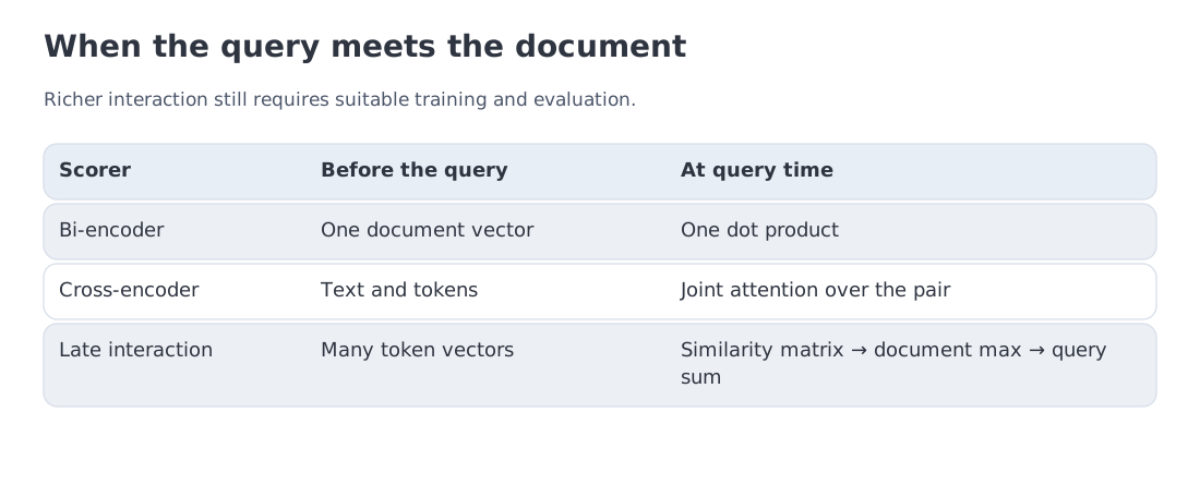 The scoring continuum: one vector per side, joint pair encoding, and token-level late interaction. Expressiveness rises together with serving cost or index size.
8. Worked example B: exact search and the arithmetic of ANN
For normalized vectors, exact cosine search is a matrix-vector product. Comparing one query with vectors of dimension requires approximately
floating-point operations.
With and :
At an illustrative sustained rate of 10 GFLOP/s, the arithmetic-only time estimate is
Now imagine that an ANN structure navigates to a shortlist requiring 2000 full vector distances. The corresponding arithmetic is
or 0.4096 ms at the same rate. The ratio of distance arithmetic is 5000.
This is deliberately not an HNSW (Hierarchical Navigable Small World) latency claim. ANN (Approximate Nearest Neighbor) search also performs graph or centroid navigation, random memory access, decompression, filtering, and candidate maintenance. Its central trade-off is not “exact search but faster”; it is less inspected state in exchange for a nonzero miss probability.
The correct benchmark therefore has at least four axes:
- recall at a chosen against an exact reference;
- latency distribution, not only the mean;
- memory including index metadata;
- update and rebuild cost.
A speed number without recall is incomplete. A recall number without a latency and memory budget is equally incomplete.
9. ANN under the hood: three indexes for three resource constraints
Approximate nearest-neighbor methods reduce the part of the vector space examined per query, but they do so in different ways.
HNSW (Hierarchical Navigable Small World): spend memory on navigable links
Hierarchical Navigable Small World graphs connect each vector to neighbors at several levels. Search begins in a sparse upper layer and descends toward denser local neighborhoods. Parameters such as construction degree and efSearch trade graph memory and query work for recall.
HNSW is attractive for low-latency in-memory search and incremental insertion. Its main tax is the graph itself: edges can occupy memory comparable to or larger than compressed vectors. Filtering and deletions also require careful implementation because the graph was built without necessarily knowing the request-time predicate.
IVF-PQ (Inverted File + Product Quantization): partition first, compress second
An inverted file index assigns vectors to coarse centroids. A query probes only several nearby lists. Product Quantization then splits a vector into subspaces and stores a small code per subvector.
nprobe controls how many coarse lists are examined; code length controls the memory/error trade-off. IVF-PQ is compelling when vector payload dominates the system budget, but it introduces centroid training, quantization error, and a more involved update path.
DiskANN: keep the large body of the index on SSD
DiskANN combines graph navigation with storage layouts designed for SSD. The original work demonstrated billion-point search on a single machine with 64 GB of RAM and SSD storage. The result does not imply that every disk-backed index beats in-memory HNSW. It addresses a different constraint: the collection is too large for the available memory.
The index algorithm and the operating model are separate decisions. ANN may live inside a library, a relational extension, a search engine, or a dedicated vector service. A database extension can simplify transactions, metadata, and access-control enforcement when the data already lives there. A separate service can offer independent scaling and specialized lifecycle management. There is no universal corpus-size threshold at which “a vector database becomes mandatory.”
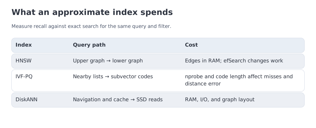 HNSW spends memory on a graph, IVF-PQ compresses and probes selected regions, and DiskANN moves the large body of the index to SSD.
10. Hybrid retrieval, reciprocal-rank fusion, and worked example F
Sparse and dense branches return scores in different units. BM25 may produce values in the teens; cosine similarity may lie near one; distributions also change from query to query. Direct score addition therefore requires calibration.
Reciprocal Rank Fusion (RRF) avoids this calibration by combining positions:
where is the one-based rank of document in branch . A missing document contributes zero. The constant softens the gap between neighboring top ranks; branch weights can express prior importance.
RRF can recover a document that appears high in either branch, but it cannot create evidence absent from both lists. It also does not inspect the query-document pair again. That is the job of a reranker.
The table uses three different views of a ranking. Recall@k is the fraction of the relevant set retrieved in the first positions: retrieving one of two relevant documents gives , even if that document ranks first. MRR averages the reciprocal position of the first relevant result, using zero when none is found. nDCG@k compares the graded value of the returned order with an ideal order. A value of one is ideal under the supplied judgments; Section 17 develops the discount and gain functions.
The offline dense branch uses Latent Semantic Analysis (LSA). It constructs a document–term TF-IDF matrix and uses singular value decomposition (SVD) to approximate it as . The retained directions have the largest singular values: they capture strong co-occurrence patterns in this matrix, rather than predefined semantic topics. Both documents and queries are projected as and normalized for cosine comparison. The resulting geometry is learned from word co-occurrence in this collection. It is a linear model without the pretrained knowledge of a large neural encoder, so paraphrase understanding is not guaranteed.
The frozen thirteen-document, seven-query English teaching collection produces these metrics:
| Method | MRR (Mean Reciprocal Rank) | Recall@5 | nDCG@5 (Normalized Discounted Cumulative Gain) |
|---|---|---|---|
| BM25 | 1.000 | 0.929 | 0.971 |
| dense LSA (Latent Semantic Analysis) proxy | 0.905 | 0.714 | 0.730 |
| RRF, | 0.929 | 0.857 | 0.855 |
| interaction reranker | 1.000 | 0.929 | 0.970 |
These are authored diagnostic documents and development queries, frozen outside the lecture. LSA is fitted to the indexed corpus without query labels. The untrained reranker averages each query word's best character-trigram Jaccard match: it does not run a neural cross-encoder or ColBERT. Since the RU and EN wording differs, the two tables do not estimate a language effect.
Here the lexical branch is already extremely strong. Adding the weaker dense ranking through RRF lowers nDCG, and the reranker mostly restores the original ordering rather than surpassing it. The Russian frozen collection shows a different pattern, where the dense branch contributes additional recall and reranking improves nDCG substantially.
The contrast is the lesson: hybrid retrieval is not guaranteed to beat every branch on every metric. Its value depends on whether branches fail on different query classes. Fusion broadens or stabilizes the candidate set; reranking re-evaluates individual pairs. They solve different problems.
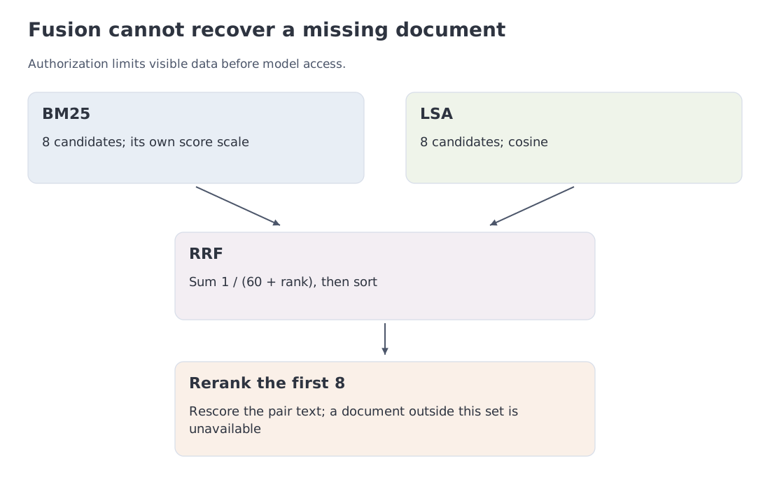 Sparse and dense branches create candidates, RRF merges positions, and an interaction reranker revisits a bounded set of query-document pairs.
11. Chunking: deciding what the index is allowed to retrieve
A retriever does not search an abstract document. It searches the units created during indexing. Chunking therefore defines the memory granularity of the whole system.
A long chunk may mix several topics into one embedding and consume too much generator context. A very short chunk may omit a definition, antecedent, table header, or causal step. The best boundary is a relevance decision, not merely preprocessing.
Fixed windows with overlap
A window of several hundred tokens with overlap is a strong baseline. It is deterministic, simple to reproduce, and easy to vary in an ablation. Overlap protects local relationships near boundaries, but increases duplicate evidence and index size.
Structure-aware chunks
Headings, paragraphs, table regions, code blocks, and page boundaries may provide more natural units. The quality then depends on parsing. A malformed PDF or inconsistent markup can produce fragments that are semantically worse than fixed windows.
Late chunking
Late chunking runs a long document through a long-context encoder first and pools contextualized token representations only afterward. A short chunk can retain information from earlier text, including antecedents and section context. The cost is a more expensive indexing pass and dependence on the encoder's maximum length. The described method needs token states and mean pooling within each chunk; a last-token-only embedding interface cannot be substituted unchanged. The authors separately study overlapping windows for longer documents, and report that gains depend on chunk size and task.
Contextual Retrieval
Anthropic's Contextual Retrieval prepends a short generated description of where a chunk sits within its source document before embedding and lexical indexing. In the company's reported experiments, contextual embeddings reduced top-20 retrieval failure by 35%; combining contextual embeddings with contextual BM25 reduced it by 49%; adding reranking yielded a 67% reduction. These are results for the stated models, corpora, and protocol, not universal multipliers.
Now take a 20-million-token corpus, chunk size 400, and overlap 64. The stride is 336, so the exact chunk count is
The count assumes one continuous document. For separate documents, sum the count per document instead of applying this equation to their combined length. Padding every window to 400 positions gives encoded positions, including overlaps and padding.
The frozen scenario estimates encoding with a 0.6B model at FLOP. At 990 TFLOP/s and MFU 0.5, the estimate is 57.7 seconds. It excludes reading, tokenization, packing, writes, retries, and orchestration.
The raw vectors occupy 232.52 MiB in fp32, 58.13 MiB in int8, and 7.27 MiB in binary form. At this corpus size, metadata, access rules, update logic, and chunk quality may dominate the vector payload itself.
12. The full cascade and worked example D: where request latency lives
Access-control lists (ACLs) must constrain visible data before text reaches any reranker or generator that lacks permission to read it. With post-filtered search, measure candidate count and recall after filtering; restricted metadata must not leak through the response.
We can now follow one request through a realistic cascade.
- Normalize the query or decompose it into subqueries.
- Run lexical and dense candidate generation.
- Merge candidates with RRF or another fusion rule.
- Rerank a bounded list.
- Remove duplicates from authorized evidence, preserve citations, and pack evidence into a token budget.
- Run generator prefill and decode.
- If evidence remains insufficient, reformulate and search again.
The assembled context crosses a trust boundary. Retrieved passages supply evidence, not authority to issue new commands. A highly ranked, correctly cited document may still contain an instruction planted by someone else. Its position in the results does not authorize a tool action. Module 18 develops this distinction in an agent loop.
The frozen scenario uses an approximately 8B generator, eight 400-token chunks, a 0.6B reranker over 100 candidates, and a 300-token answer.
The timing assumptions need to be visible before the stages are added. For the encoder and reranker, approximate forward work as , with parameters and processed tokens. A peak rate of 990 TFLOP/s and an assumed MFU of 0.5 give a modeled rate of FLOP/s. The query has 32 tokens, so its estimate is ms. One hundred query–chunk pairs contain tokens and require 104.7 ms under the same model.
The generator has exactly parameters in this calculation. Its input consists of 512 instruction/query tokens plus eight 400-token chunks, giving 3712 and a linear prefill estimate of 120.4 ms. Decode uses a separate assumed rate of 209.4 tokens/s: s. That rate was neither measured here nor derived from .
Adding the stages assumes serial execution. Queuing, networking, index reads, and packing are omitted. MFU need not be equal for a tiny query and a batch of pairs; attention's quadratic work is also omitted. This makes the table a conditional scenario budget, not a rigorous request-latency lower bound.
| Stage | Conditional time estimate | Share of total |
|---|---|---|
| query encoding | 0.0776 ms | <0.1% |
| 2000 full distances after ANN navigation | 0.4096 ms | <0.1% |
| rerank 100 candidates | 104.7 ms | 6.3% |
| prefill 3712 tokens | 120.4 ms | 7.3% |
| decode 300 tokens | 1432.7 ms | 86.4% |
| total | 1.658 s | 100% |
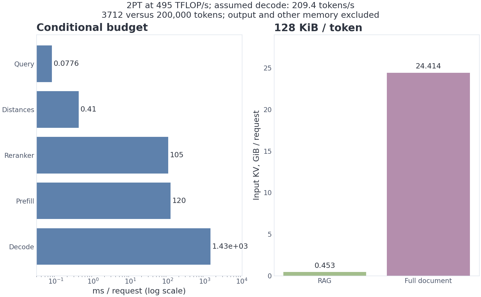 Left: a parameterized cascade budget. Right: the same input-length factor appears in prefill and KV memory in the teaching comparison of RAG and a full document.
The table does not establish that reranking is generally cheap. It shows that one long-answer interactive scenario is dominated by decode. Short answers, a larger rerank set, a remote API, or saturated batch generation can move the bottleneck elsewhere.
The correct optimization sequence therefore begins with measurement. A team may need to accelerate generation, reduce candidate count, cache query embeddings, or simplify retrieval. The 6.34% retrieval-before-prefill share belongs to this scenario only.
13. Level-1 code: hybrid retrieval with explicit contracts
The two functions below expose different sources of evidence. RRF reads ranks and combines their contributions without inspecting text. MaxSim forms a token-similarity matrix, then chooses the strongest document match for each query token. Token vectors arrive normalized; this example does not train an encoder.
"""RRF and exact late interaction: executable, model-independent mechanisms."""
import numpy as np

def rrf(rankings, k=60):
    """Accumulate one-based reciprocal ranks, then sort U unique candidates."""
    if not np.isfinite(k) or k <= 0:
        raise ValueError("k must be positive and finite")
    scores = {}
    for ranking in rankings:
        if any(not isinstance(doc, str) or not doc for doc in ranking):
            raise ValueError("IDs must be nonempty strings")
        if len(ranking) != len(set(ranking)):
            raise ValueError("duplicate document in a branch")
        for rank, doc in enumerate(ranking, 1):
            scores[doc] = scores.get(doc, 0.0) + 1.0 / (k + rank)
    return sorted(scores, key=lambda doc: (-scores[doc], doc)), scores

def maxsim(query, document):
    """Q:[nq,d], D:[nd,d]; sum the best document match for each query row."""
    q, d = np.asarray(query, float), np.asarray(document, float)
    if q.ndim != 2 or d.ndim != 2 or q.shape[1] != d.shape[1]:
        raise ValueError("expected two matrices with one shared feature dimension")
    if not all(q.shape) or not all(d.shape):
        raise ValueError("empty token matrices")
    if not np.isfinite(q).all() or not np.isfinite(d).all():
        raise ValueError("non-finite vectors")
    if not (np.allclose(np.linalg.norm(q, axis=1), 1)
            and np.allclose(np.linalg.norm(d, axis=1), 1)):
        raise ValueError("normalize token vectors before cosine MaxSim")
    similarities = q @ d.T
    return float(similarities.max(axis=1).sum()), similarities

order, scores = rrf([["a", "b"], ["b", "c"]])
assert order == ["b", "a", "c"]
assert np.isclose(scores["b"], 1 / 62 + 1 / 61)
score, matrix = maxsim(np.eye(2), np.array([[1.0, 0.0]]))
assert score == 1.0 and matrix.shape == (2, 1)
Document b receives two reciprocal-rank contributions and moves ahead of both single-branch documents. In the MaxSim example, one query vector matches the sole document vector and the other is orthogonal, so the sum is one. Several query tokens may choose the same document token: MaxSim imposes no one-to-one assignment.
Accumulation is linear in the total input-list length. Sorting the unique candidates adds work. The notebook surrounds these mechanisms with indexing, validation, metrics, and provenance checks.
15. The evolution of RAG: repair the measured failure, not the acronym list
“Advanced RAG” is most useful when understood as a set of repairs.
If a short question embeds poorly because relevant documents are written in answer form, HyDE (Hypothetical Document Embeddings) generates a hypothetical answer and searches with its representation. The method changes the query side of the mismatch.
If one retrieval pass is sometimes unnecessary and sometimes insufficient, Self-RAG adds retrieval and critique decisions to generation. The model can decide whether evidence is needed and evaluate what it receives.
If retrieved evidence may be weak or misleading, CRAG (Corrective Retrieval-Augmented Generation) introduces a retrieval-quality evaluator and a fallback path. The repair is not a new index; it is a decision about whether to trust the current candidates.
If the answer depends on information at several scales, RAPTOR (Recursive Abstractive Processing for Tree-Organized Retrieval) builds a hierarchy of recursive summaries. Fine chunks and higher-level summaries become retrievable units.
If the question is global—“what themes or relationships characterize this corpus?”—plain top- chunks may not contain a sufficient view. GraphRAG builds entity and relationship structures plus community summaries to support corpus-level synthesis. That capability comes with higher indexing cost and more model-generated intermediate state.
The next step is agentic retrieval. Search becomes one tool in a loop: formulate a query, inspect results, follow a lead, reformulate, and stop when evidence is sufficient. The gain is adaptive multi-hop behavior. The price is variable latency, cost, and a larger failure surface.
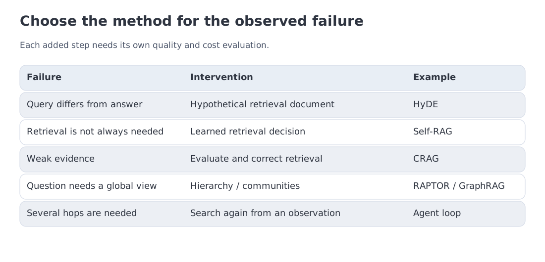 Each family addresses a distinct failure: query mismatch, uncertain evidence, missing hierarchy, global corpus questions, or the need for iterative search.
The design rule is intentionally conservative: add the smallest mechanism that fixes an observed error. If BM25 plus a reranker already satisfies the task, a graph and an autonomous loop may add cost without adding evidence.
16. Worked example E: RAG or long context
Suppose the complete document contains 200,000 tokens, while retrieval and context assembly produce 3,712 tokens. The length ratio is
Under the same linearized prefill model, the full document requires 6.4889 seconds and the RAG context 0.120434 seconds. With a KV cost of 128 KiB per token, the payloads are
for the full document and
for the RAG context. The same ratio appears because the scenario holds architecture and bytes per token constant.
The equal ratios follow from the linear approximation. Attention's quadratic work may matter at 200,000 tokens. Constant KV bytes per position assumes unchanged architecture and precision. These payloads count input KV only, excluding the future answer and other runtime memory.
This arithmetic does not make RAG universally superior. Long context preserves document order, global structure, and evidence that may not be individually retrievable. It can be preferable when one or a few documents must be read as wholes, when queries are global, or when retrieval recall is difficult to guarantee.
RAG is attractive when the corpus is much larger than one request's evidence needs, changes frequently, requires access control, or must provide citations. It pays an indexing and retrieval tax in exchange for a much smaller generator input.
Research comparing RAG and long context finds the same qualitative split: with enough resources, long-context models can be stronger on average for some tasks; RAG is usually cheaper; routing between them can approach long-context quality while avoiding its cost on every query. The correct policy is therefore often conditional rather than ideological.
A router can use cheap features—document count, requested scope, retrieval confidence, question type, or a learned classifier—to choose retrieval, full context, or a hybrid path. The router itself must be evaluated because a wrong route can be more expensive than a modestly suboptimal retriever.
17. Evaluation and the embedder passport
A RAG evaluation should identify the stage that failed.
Retrieval metrics
- Recall@k asks whether the relevant set survived candidate generation.
- MRR emphasizes the first relevant item.
- nDCG@k rewards good ordering when relevance is graded.
These metrics require relevance judgments and an explicit unit of retrieval. Page-level, chunk-level, and document-level judgments are not interchangeable.
To make nDCG reproducible, define both gain and discount. Let be the integer relevance grade at rank :
IDCG sorts all known grades before taking the first . With grades 3 and 1, the ideal value is . Reversing the documents gives . Recall@2 remains one, and reciprocal rank remains one too: the first item is still relevant. Graded ordering, completeness, and the first useful result are distinct properties.
The notebook rejects a query with no positive judgments instead of silently reporting zero. Such queries belong in a real evaluation of abstention, but need an explicit protocol. Rankings must not repeat an ID, since duplicated gains can inflate nDCG above one. Aggregation gives every query equal weight, regardless of how many documents it retrieves.
Generation metrics
- groundedness or faithfulness to retrieved evidence;
- citation correctness and completeness;
- answer relevance and task success;
- refusal behavior when evidence is insufficient.
A high retrieval recall with poor groundedness points toward generation or context assembly. A polished answer with low retrieval recall may be unsupported even if it sounds correct.
System metrics
Latency should be split into query encoding, ANN, filtering, reranking, context assembly, prefill, and decode. Track memory, index build time, update lag, failure rate, and cache hit rate where relevant. Tail latency matters for agent loops because one slow retrieval can delay the entire trajectory.
Public suites help form a shortlist. BEIR (Benchmarking IR) evaluates zero-shot retrieval across heterogeneous tasks; MTEB (Massive Text Embedding Benchmark) broadens embedding evaluation; MMTEB (Massive Multilingual Text Embedding Benchmark) extends coverage to more than 500 tasks and more than 250 languages. A leaderboard score still does not describe the target corpus, query style, chunk size, language mixture, instruction format, or latency budget.
A useful embedder passport records:
- model revision and license;
- vector dimension and whether shorter vector prefixes were trained as usable representations (MRL, Section 6);
- tokenizer, maximum length, pooling, and normalization;
- query/document instructions or prefixes;
- supported languages and domains;
- retrieval unit and chunking method used in evaluation;
- dense index and precision;
- metrics on the local judged query set;
- hardware, batch size, and measured latency.
Qwen3 Embedding is one example of why the passport matters: the family includes 0.6B, 4B, and 8B embedding and reranking models under Apache 2.0. The model name alone does not tell a system which size, dimension, instruction, precision, or reranker was used.
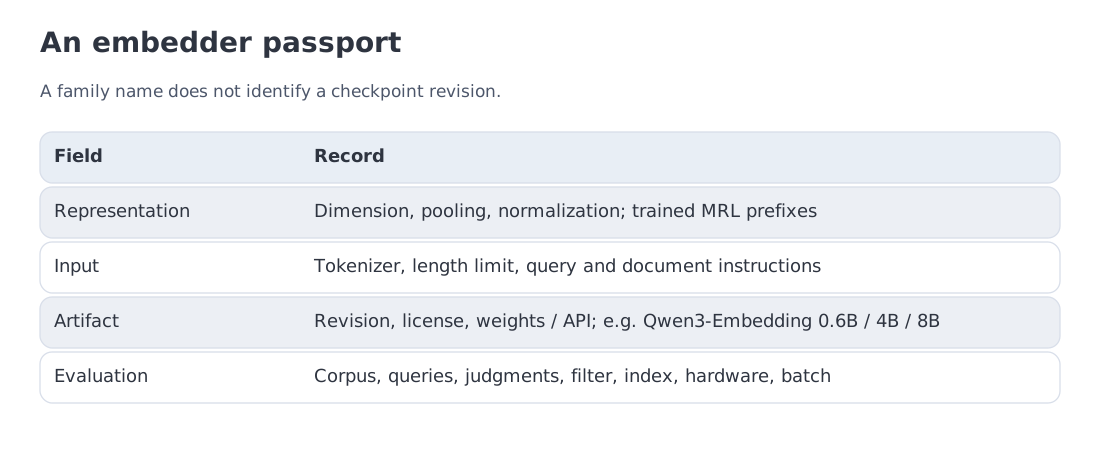 An embedder passport connects the checkpoint to tokenization, pooling, instructions, dimensionality, corpus, metrics, index, and measured hardware.
20. Key takeaways and sources
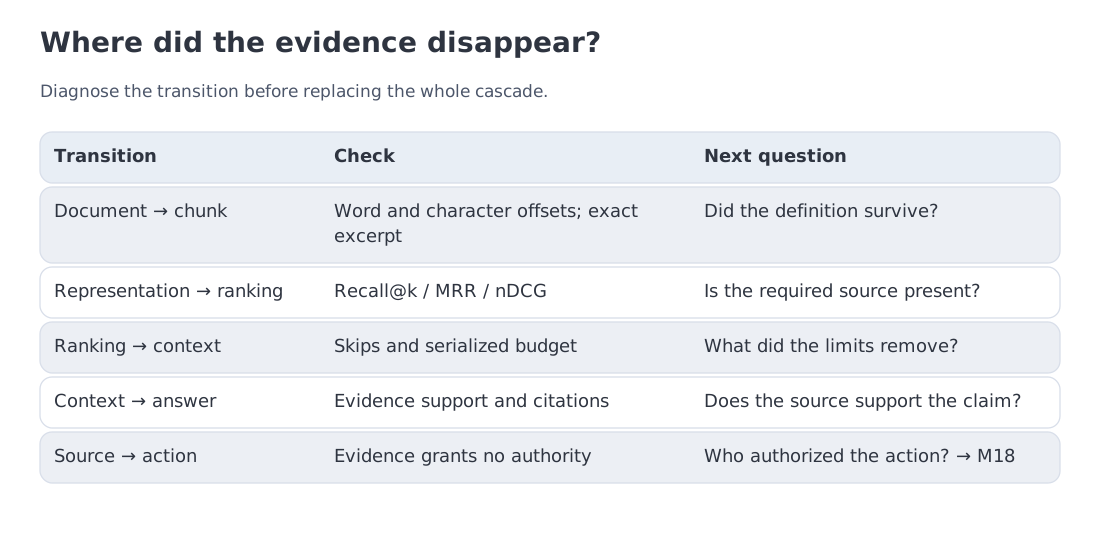 The module in one map: four information losses, three scoring architectures, ANN, fusion and reranking, chunking, context assembly, and stage-wise evaluation.
A RAG request passes through a cascade in which every stage reduces information.
Lexical retrieval preserves rare literal terms when the analyzer retains the required distinctions. BM25 combines corpus rarity, term-frequency saturation, and document-length normalization. Learned sparse models add semantic expansion while retaining inverted-index execution.
Dense retrieval represents text as vectors. Its quality depends on negatives, instructions, pooling, language, and domain. One-vector search scales well but compresses token structure early.
Cross-encoders and late interaction restore richer interaction. A cross-encoder is suited to a bounded pair list; late interaction keeps multiple document vectors and pays with a larger index.
MRL and quantization control storage. MRL trains useful prefixes of one vector (Section 6); quantization reduces bits per retained coordinate. Ten million 1024-dimensional vectors range from 38.15 GiB in fp32 to 1.19 GiB as a raw binary payload, before index metadata.
ANN reduces inspected state and introduces miss probability. HNSW, IVF-PQ, and DiskANN spend memory and storage differently; none is selected by corpus size alone.
Fusion and reranking have different responsibilities. RRF combines positions without score calibration; a reranker revisits actual pairs. On the frozen teaching set, fusion does not beat BM25 on nDCG, while reranking improves the final order.
Chunking defines the retrievable memory unit. Overlapping windows are a strong baseline; late chunking and contextual retrieval restore document context at additional indexing cost.
RAG and long context are conditional tools. RAG reduces input and supports freshness, access-control lists (ACLs), and citations. Long context preserves a document's global structure. Routing can choose per request.
Evaluation must remain stage-wise. Recall, MRR, and nDCG diagnose retrieval. Groundedness, citation quality, and task success diagnose generation. An embedding leaderboard is a shortlist, not a deployment decision.
Primary sources
- Gao et al., HyDE — arxiv.org/abs/2212.10496
- Yan et al., CRAG — arxiv.org/abs/2401.15884
- Lewis et al., RAG — arxiv.org/abs/2005.11401
- Karpukhin et al., DPR — arxiv.org/abs/2004.04906
- Khattab & Zaharia, ColBERT — arxiv.org/abs/2004.12832
- Formal et al., SPLADE — arxiv.org/abs/2107.05720
- Wang et al., E5 — arxiv.org/abs/2212.03533
- Kusupati et al., MRL — arxiv.org/abs/2205.13147
- Malkov & Yashunin, HNSW — arxiv.org/abs/1603.09320
- Subramanya et al., DiskANN — NeurIPS 2019
- Faysse et al., ColPali — arxiv.org/abs/2407.01449
- Zhang et al., Qwen3 Embedding — arxiv.org/abs/2506.05176
- Günther et al., Late Chunking v3 — arxiv.org/abs/2409.04701v3
- Anthropic, Contextual Retrieval — anthropic.com/engineering/contextual-retrieval
- Asai et al., Self-RAG — arxiv.org/abs/2310.11511
- Sarthi et al., RAPTOR — arxiv.org/abs/2401.18059
- Edge et al., GraphRAG — arxiv.org/abs/2404.16130
- Li et al., RAG versus long context / Self-Route — arxiv.org/abs/2407.16833
- Thakur et al., BEIR — arxiv.org/abs/2104.08663
- Muennighoff et al., MTEB — arxiv.org/abs/2210.07316
- Enevoldsen et al., MMTEB — arxiv.org/abs/2502.13595
- Es et al., Retrieval-Augmented Generation Assessment (RAGAS) — arxiv.org/abs/2309.15217
Next: Module 18 studies the agent that treats retrieval as one tool among many: it plans an action, calls an environment, observes the result, and decides whether to continue.
Landscape verified: 11 October 2026. Storage and latency values are reproducible module scenarios, not measurements of a particular vector engine or production service.