Module 8. Beyond the Transformer: SSMs, Mamba, and Hybrid Sequence Models
“Modern LLMs” course · Module 8 lecture · edition 2026.10.25
What this module is about. Softmax attention keeps the past as an addressable KV cache. That preserves separately addressable positions, but the cache grows with every token. A State Space Model (SSM) takes the opposite bargain: after each token, update a fixed-size state. We will start from a continuous linear system and exact Zero-Order Hold discretization, then move through Mamba selectivity, Mamba-2’s State Space Duality, delta-rule memories, and current hybrid architectures. The recurring question is not whether recurrence “beats” attention. It is which parts of the past can be compressed into a fixed state, and which still require an addressable store.
Prerequisites. Module 5 introduced KV-cache geometry; Module 6 covered the residual block; Module 7 is useful for the MoE hybrids later in the lecture. Everything needed for the argument is restated here.
Reading routes
First pass: §1 → §§3–4 → §§6–11 → §§17 and 19. In §4, first understand the discrete recurrence and its matrices; save the exact-coefficient derivation and E1 in §18 for the second pass. E2–E3 provide the first memory calculations. Follow the change from a list of past tokens to a fixed state, then study writing, forgetting, and hybrids. Return to the opening memory figures when you reach §10.
Second pass: §§4–5, §7, and §§12–14 with the notebook. Derive the discrete update and test composition, chunk boundaries, and numerical limits.
Reference pass: §2, §15, and §20 provide history, model specifications, and sources. They introduce names as pointers; the mechanisms are developed in §§3–11.
1. Two costs of a long context
A Transformer pays for length in two related but different places. During dense prefill, attention considers token pairs and its central arithmetic is quadratic in sequence length. During autoregressive decode, each new query reads the accumulated keys and values, so both per-step work and cache size grow with the preceding context.
An SSM stores history in another form:
where has a fixed shape. Processing a sequence remains linear in length, and the recurrent cache does not expand as the conversation continues.
That resource win is not free. A KV cache resembles an indexed collection: a later query can point back to a specific record. A recurrent state is closer to a continuously rewritten summary. It can preserve the statistics that training makes useful, but independent facts may interfere, and arbitrary exact retrieval does not come for free.
Our first memory calculation already shows why the alternative matters. For a 32-layer Mamba-style stack with , , a convolution width of four, and bf16 state, the main SSM cache is 8 MiB and the causal-convolution cache another 2 MiB. The complete fixed cache is therefore 10 MiB. A reference Transformer cache at 128 KiB per token reaches the same size after only 80 tokens.
For a Mamba-2-like teaching geometry with , the complete cache is 66.0625 MiB. The exact crossover is 528.5 tokens; token 529 is the first integer position beyond it. These values are not universal model constants. They demonstrate why the cache contract must include every persistent state, not only the tensor named ssm_state.
2. From control theory to hybrid language models
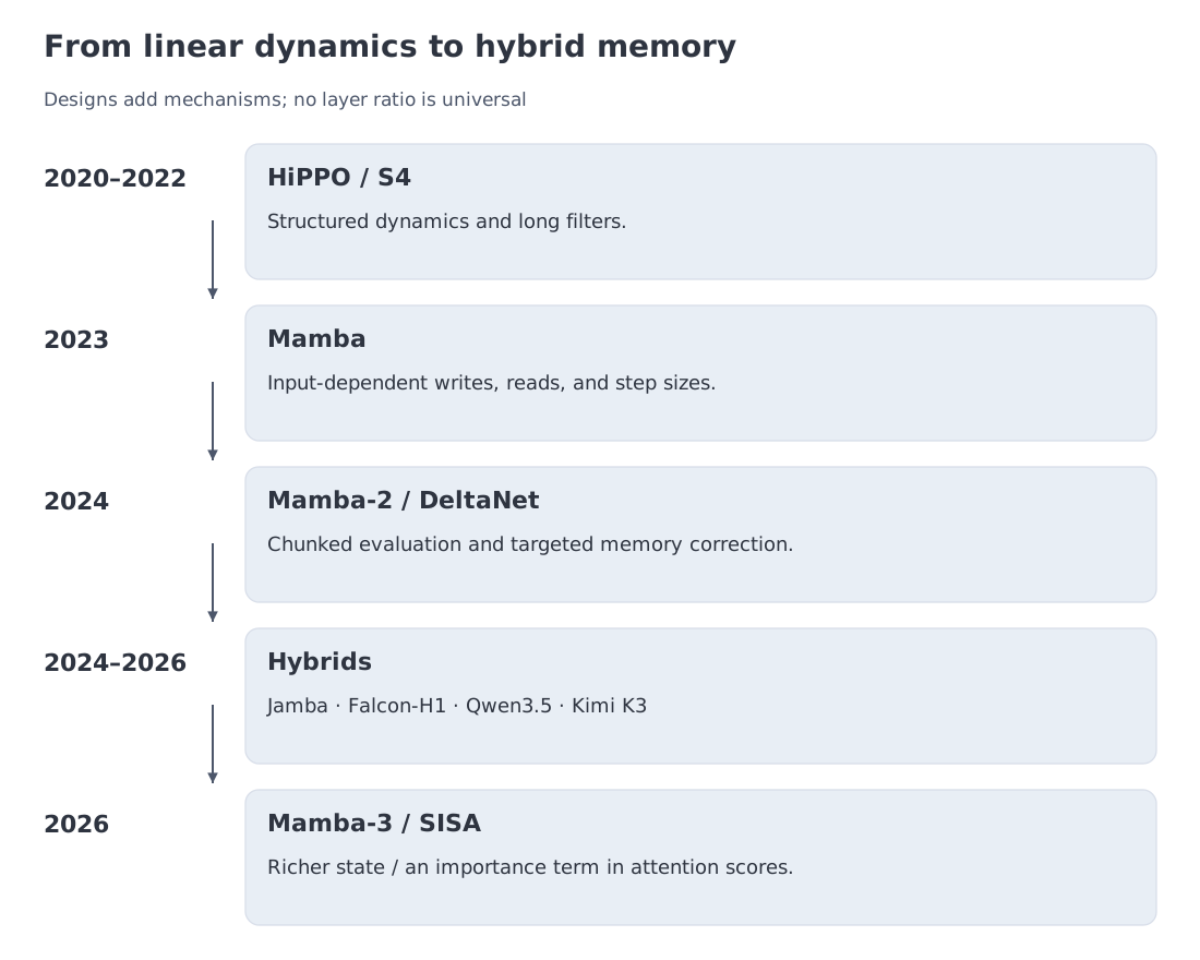 Classical state-space systems → HiPPO/S4 → selective Mamba → Mamba-2/SSD and DeltaNet → Jamba, Falcon-H1, Qwen3.5, and Kimi hybrids → new recurrent and sparse branches in 2026.
State-space systems long predate neural language models. In control and filtering, a compact hidden state is designed to retain what is needed for future prediction. S4 — Structured State Spaces for Sequence Modeling brought that idea into deep sequence models and used structured dynamics to make very long convolutions tractable.
The weakness of early learned SSMs was not simply memory length. Their update law changed too little with content. Mamba made the input map, output map, and effective step size depend on the current token. The model could now decide that one symbol should be recorded strongly while another should pass with little effect. A hardware-aware selective scan made this input-dependent recurrence practical on GPUs. The paper reports up to a fivefold throughput improvement over its compared Transformer configurations; that is a result of the authors’ implementation and protocol, not a generic multiplier for every stack.
Mamba-2 introduced State Space Duality (SSD). For a structured class of transitions, the same sequence operator can be expressed as a recurrence or as a semiseparable masked matrix closely related to linear attention. This opened a path to dense matrix work inside chunks while carrying only compact state across chunk boundaries. The authors report a 2–8× core-layer speedup over Mamba-1 in their settings.
In parallel, linear-attention research revisited how memory should be written. The June 2024 DeltaNet paper developed efficient parallel training for a memory that uses the delta rule to correct an existing association rather than merely adding another outer product. Gated DeltaNet, published later in December 2024, combined that mechanism with adaptive forgetting.
Large systems then converged on hybrids rather than one universal replacement. Jamba interleaved Transformer, Mamba, and MoE components. Falcon-H1 ran Mamba-2 and attention in parallel. Qwen3.5 used three Gated DeltaNet layers followed by one full-attention layer in each repeated unit. Kimi K3 combined 69 KDA layers with 24 Gated MLA layers. The recurring design lesson is more durable than any one ratio: fixed state is attractive as a low-cost carrier, while addressable mechanisms are retained where compression is not enough.
3. Three readings of the same recurrence
A dynamical system
A continuous linear SSM is
controls internal evolution, writes the input, reads the state, and provides a direct input-to-output path.
The state , input , and output fix the matrix shapes: , , , and . The dot denotes a continuous-time derivative; tokens will instead index discrete updates.
A bank of temporal filters
If every eigenvalue of has a negative real part, the unforced state tends to zero over time: the system is asymptotically stable. This does not require each coordinate to decrease monotonically; a general matrix can produce transient growth. In the diagonal examples below, individual negative coefficients directly set different decay times. The system can then be read as a bank of fast and slow temporal filters.
An associative memory
A linear-attention memory is often written as
The key selects a write direction, the value provides the content, and the query reads from the resulting matrix. Unlike an explicit KV table, the matrix has fixed size, so independent associations eventually interfere.
For the associative form, , , and . The outer product writes one association; multiplication by the query reads a value-sized vector. This is unnormalized linear attention, with no softmax.
These views are complementary. Dynamics explains stability and forgetting; filters explain time scales; associative memory explains writing and retrieval. Mamba-2 makes the connection more than rhetorical for its structured class of operators.
4. Discretization with Zero-Order Hold
Language arrives at discrete positions, so a continuous system must be discretized. Under Zero-Order Hold (ZOH), the input is treated as constant for an interval of duration :
The bars distinguish one-step discrete matrices from the continuous system: propagates the previous state, while adds the current input. This recurrence is the starting point for reading Mamba. The following equations derive its coefficients for a specified continuous-time system.
For invertible , the integral equals . The integral also covers singular matrices. The numerical examples set the direct path to zero.
For diagonal , the calculation is elementwise. When one diagonal entry is zero, the expression for looks singular, but the limit is well defined:
The module code handles that limit explicitly so a rare zero mode cannot create a hidden NaN.
The exact ZOH formula and a production Mamba parameterization are not the same object. In the open Mamba-2 implementation, the input update uses a term of the form inside its efficient formulation rather than materializing the exact ZOH input matrix above. The continuous model supplies intuition; the architecture chooses a trainable discrete update that can be implemented efficiently.
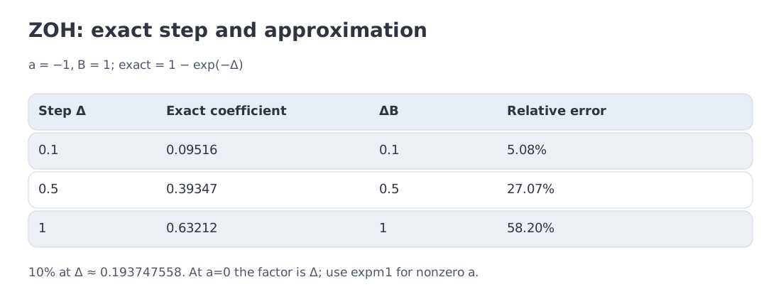
5. Worked example: the cost of replacing exact ZOH by
Take one stable scalar mode:
The exact input coefficient is
while the small-step approximation is . Its relative error is
| exact | approximation | relative error | |
|---|---|---|---|
| 0.1 | 0.09516 | 0.1 | 5.08% |
| 0.5 | 0.39347 | 0.5 | 27.07% |
| 1.0 | 0.63212 | 1.0 | 58.20% |
Solving
gives
The point is not that every selective SSM must implement full ZOH. It is that and the exact held-input coefficient are distinct claims; a lecture or codebase should say which one it uses.
 An exact two-mode ZOH trace, the zero-eigenvalue limit, and the growth of the approximation error.
6. What selectivity changes in Mamba
A time-invariant linear system applies the same write and forgetting law to every symbol. Language needs content-dependent control. Mamba predicts write and read maps and a positive step from the current input. Here ensures a positive step; the expression is schematic:
controls writing, controls reading, and changes the effective rate at which the state moves. A token can therefore preserve the previous state, overwrite part of it, or expose a different projection to the next block.
A short depthwise causal convolution appears before the selective recurrence. It is best understood as an explicit local inductive bias, not as evidence that recurrence cannot represent order. The convolution handles nearby patterns cheaply; the SSM carries longer dynamics.
That local path also owns persistent state at decode time. A serving implementation must keep both the SSM tensor and the convolution tail. Any memory estimate that counts only the first is incomplete.
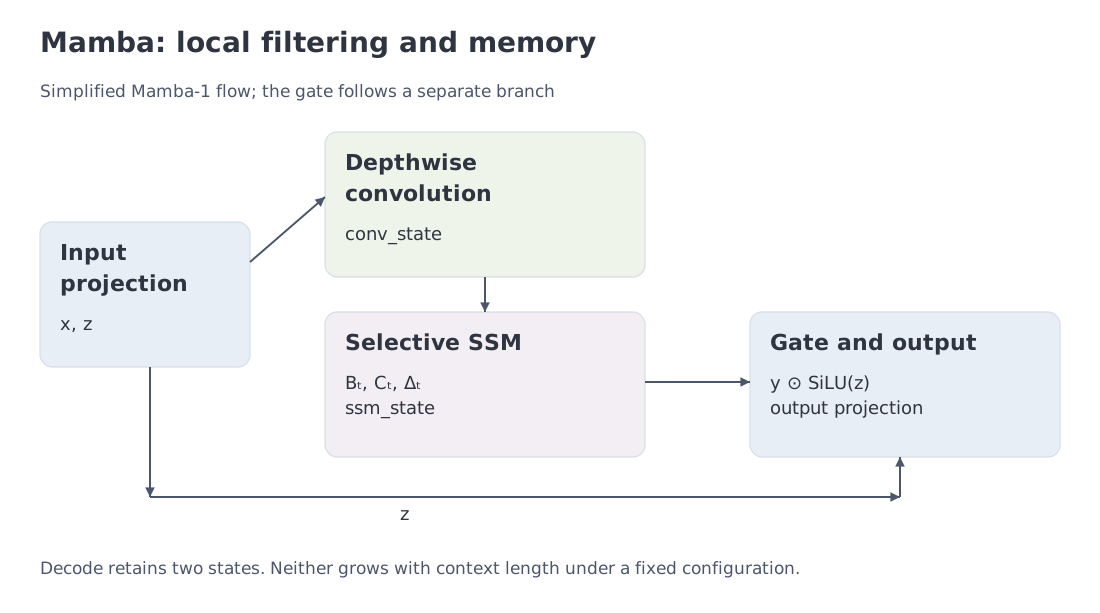 Input projection splits a local path and a gate; convolution feeds the selective SSM, whose output is multiplied by the gate. The two persistent caches are shown separately.
7. Mamba-2 and the scope of State Space Duality
Mamba-2 focuses on a structured class of state transitions whose sequence matrix is semiseparable. The same operator can then be evaluated as:
- a sequential recurrence;
- an associative parallel scan;
- a chunked matrix computation resembling masked linear attention.
A scan computes every prefix state, not just the final state. Represent the affine step by . Composition gives
Associativity permits regrouping, not reordering: followed by yields , whereas the reverse order yields .
For this representation, take scalar input and output , state , and vectors . Readout is ; the vector represents the readout row used in §3. With transition and zero initial state, the coefficient mapping input to output is
The transition product carries the write forward. Off-diagonal blocks factor through the compact state; this low-rank structure is the useful meaning of semiseparable. Matrix operations handle a chunk internally, and only the boundary state must cross to the next chunk.
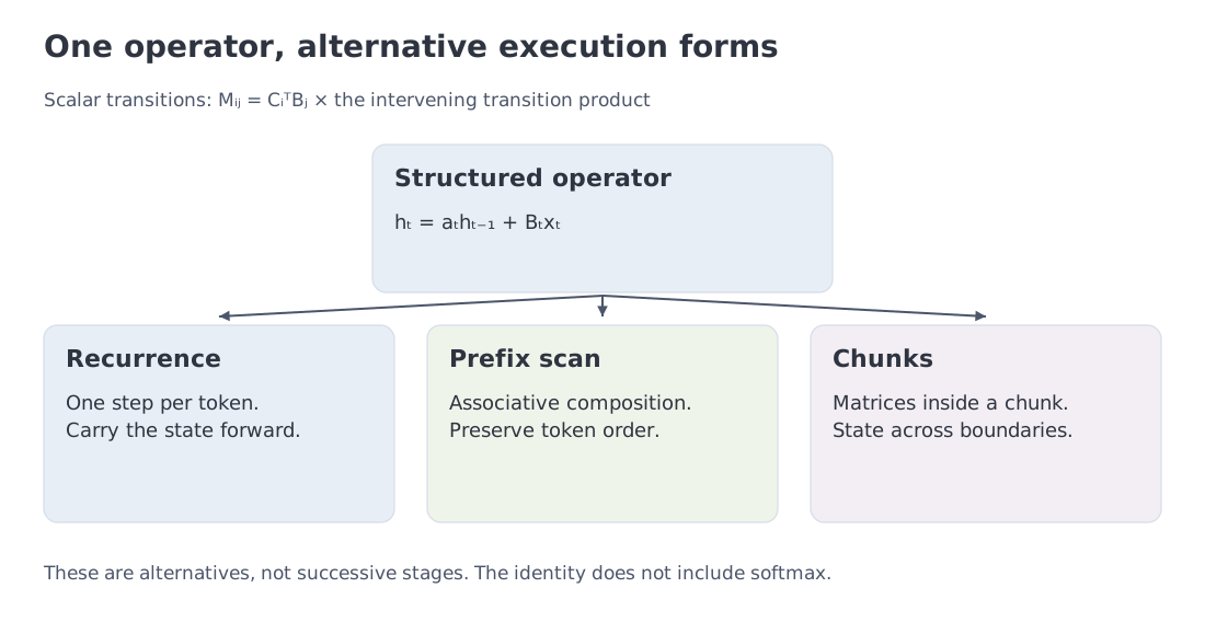 One structured operator, three execution forms. SSD is a duality for a defined class, not an identity between every SSM and every linear-attention method.
The distinction matters. The slogan “Transformers are SSMs” does not mean any arbitrary continuous dynamical system is interchangeable with standard softmax attention. The theorem relies on a specific structured matrix class.
Nor should numerical equivalence be confused with bitwise equality. A recurrence, a scan, and a GEMM-based chunked implementation can evaluate the same mathematical operator while accumulating floating-point error in different orders.
The systems advantage is phase-dependent. Chunked dense work is attractive during training; recurrence is attractive during decode. The cited 2–8× improvement concerns the Mamba-2 core layer in the paper’s measured settings, not the total latency of every model built around it.
8. Delta-rule memory and adaptive forgetting
An additive memory writes
Reusing a key adds the new value to the old one. Delta rule instead corrects the current prediction:
For a normalized key and , the readout along that direction becomes exactly . A between zero and one performs a partial update. Earlier work had already used the delta rule for associative memory.
Let
After writing , a second additive write would return for the same key. Delta update returns at and exactly at .
DeltaNet develops this form of targeted correction and a parallel training algorithm. Gated DeltaNet adds a separate forgetting gate. The mechanisms solve different problems: delta update repairs a selected association; gating can erase broader old content.
Let control global forgetting. Decay precedes the targeted correction:
For a unit key the readout is , so replaces it exactly even when . Other non-orthogonal key directions can change too; a targeted update does not make all associations independent.
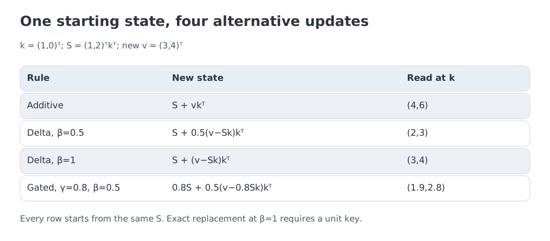 Additive write, partial correction, exact replacement, and a gated update for one key direction.
9. What a fixed state can and cannot preserve
Consider a deliberately simple associative memory:
Random normalized keys are not mutually orthogonal, so cross terms accumulate. In the frozen scenario with , mean squared error rises from roughly 0.14 at four stored pairs to about 4.14 at 128.
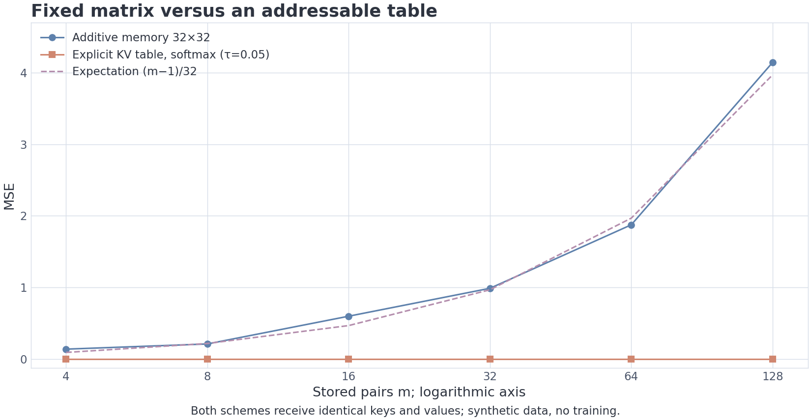 Interference in a toy additive linear associative memory. This is not a Mamba benchmark and not a theorem about every SSM.
A low-temperature softmax control (temperature 0.05, or a logit multiplier of 20) nearly recovers the explicit values in this synthetic setup because it retains the whole key/value table. That does not prove that every Transformer retrieves perfectly; it isolates the difference between an addressable table and fixed-size compression.
The defensible conclusion is:
at fixed numerical precision, fixed state creates an information bottleneck; retrieval quality depends on state size, state structure, the update rule, training, and the task.
Newer models such as Mamba-3 increase recurrent expressivity and improve state tracking in their experiments. They can shift the frontier without turning finite state into an unbounded exact database.
The plotted methods share the same random keys and values at each load. For independent isotropic unit keys in dimensions and independent zero-mean, unit-variance value coordinates, expected additive-memory MSE per coordinate is . The dashed line shows that expectation, not a claim that one seeded sample must equal it.
10. Memory accounting and core-only arithmetic
Complete recurrent cache
All sizes below cover one sequence and the stated layer stack, excluding model weights and workspaces. Let count layers, count KV heads, be head width, and be bytes per value. Use , , , and . The recurrent geometry uses channels, state coordinates per channel, and a stored convolution width . Here K=1024 and M=1024² tokens.
For the reference Transformer:
For the Mamba-1-like stack:
For the Mamba-2-like geometry, use : MiB. The open implementation can cache x plus B/C channels. With one B/C group, this gives convolution channels and MiB:
The exact crossover is 528.5 tokens, and the first integer position after it is 529.
A 32-layer hybrid with four attention layers at 256K context retains 4 GiB of KV cache plus 8.75 MiB of recurrent state in the other 28 layers. The memory remains because some layers still keep token-addressable records; the coefficient is simply much smaller.
Central operator arithmetic
Count one layer at one decode step. Set , , and , returning to the Mamba-1-like state width for this separate arithmetic example. Let be the number of visible keys. Count a multiplication and an addition as two operations, even if hardware fuses them.
Attention performs QK dot products and a weighted sum of V, each costing approximately operations. For a diagonal SSM with its coefficients already available, costs two multiplications and one addition per state coordinate. The readout contributes approximately two more operations per coordinate. Thus the leading estimates are
giving ratios of 25.6× at 1K, 819.2× at 32K, and 26,214.4× at 1M. An exact scalar count uses one fewer readout addition per channel; the leading estimate drops that small correction. These are restricted arithmetic comparisons. They exclude SSM coefficient preparation, softmax, projections, convolution, gates, FFNs, weight movement, and execution efficiency, so they do not predict whole-model speed.
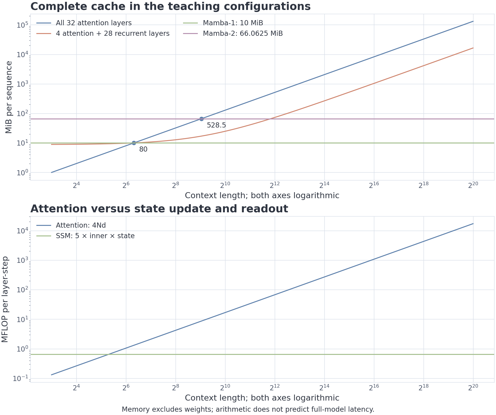 Top: complete recurrent cache versus a growing KV cache. Bottom: central token-mixing arithmetic only, not end-to-end latency.
The Mamba-2 example assumes one B/C group and all 8192 channels assigned to the SSM. More generally, convolution has channels for groups. SSM and convolution states may use different dtypes; using bf16 for both is a scenario assumption.
11. Three hybrid patterns
Interleaved layers
Jamba interleaves Transformer, Mamba, and MoE components. Qwen3.5-35B-A3B documents an exact repeating pattern:
Seventy-five percent of the layers therefore carry recurrent or linear state, while one quarter retains a full-attention cache.
Parallel branches
Falcon-H1 runs Mamba-2 and attention within the same block. This lets addressable and compressed representations interact at every depth, but it also executes the attention branch more frequently. Ablations of a trained checkpoint can reveal strong specialization between branches, yet they do not establish a universal role assignment for every hybrid architecture.
Specialized mixtures
Kimi K3 has 93 layers: 69 Kimi Delta Attention layers and 24 Gated MLA layers. Attention Residuals is a separate depth-mixing mechanism, not the name of the MLA branch. Nemotron 3 Super and Ultra combine Mamba, attention, LatentMoE, and multi-token prediction at different scales—120B/12B and 550B/55B.
MiniMax demonstrates why family names are not architecture passports. MiniMax-01 and M1 used Lightning Attention. MiniMax M2 moved to full attention after the company reported inadequate long-context quality from the hybrid alternative in its experiments. MiniMax M3 later introduced MiniMax Sparse Attention, a sparse-attention branch rather than a fixed recurrent state.
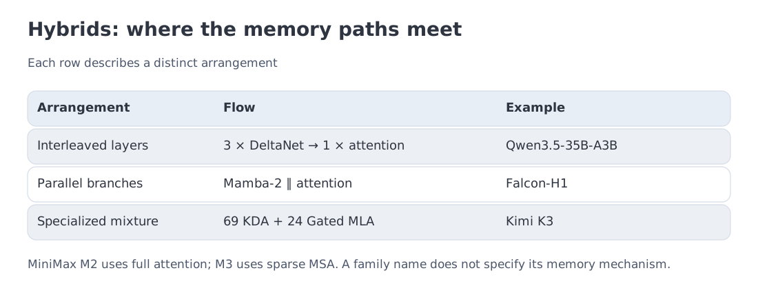 Interleaved stacks, parallel branches, and specialized hybrids. Layer ratios are checkpoint properties, not universal standards.
12. Level-1 code: exact discretization, delta update, and scan composition
import numpy as np

def zoh_diagonal(a, b, delta):
    """Diagonal A: [n], B: [n,p], positive scalar step; caller validates shapes."""
    a = np.asarray(a, dtype=np.float64)
    b = np.asarray(b, dtype=np.float64)
    transition = np.exp(delta * a)
    factor = np.full_like(a, float(delta))
    np.divide(np.expm1(delta * a), a, out=factor, where=a != 0)
    return transition, factor[:, None] * b

def delta_step(state, key, value, beta, decay=1.0):
    """State [dv,dk], unit key [dk], value [dv]; decay before correction."""
    base = decay * state
    prediction = base @ key
    return base + beta * np.outer(value - prediction, key)

def compose_affine_pair(later, earlier):
    """Elementwise transforms; returns later(earlier(h)), not the reverse."""
    a2, b2 = later
    a1, b1 = earlier
    return a2 * a1, a2 * b1 + b2
The functions represent three different claims. The first is exact discretization of a stated continuous system. The second is an editable matrix memory. The third supplies the associative operator required for a parallel scan.
A production kernel adds batched shapes, input-dependent parameters, fused causal convolution, Tensor Core layouts, and precision engineering. The teaching implementation is intentionally transparent rather than fast.
14. Reading the open Mamba implementation
A Mamba-1 inference cache commonly contains:
conv_statewith a shape like[batch, d_inner, d_conv];ssm_statewith shape[batch, d_inner, d_state].
Mamba-2 stores SSM state as [batch, nheads, headdim, d_state], where nheads * headdim = d_ssm. Convolution channels can include x plus B/C components, with width d_ssm + 2 * ngroups * d_state. These shapes and the number of groups determine the cache; the headline d_state alone is insufficient.
The source code also separates mathematical inspiration from executed update. Mamba-2’s efficient input branch uses a term. A source audit should therefore ask both:
- which continuous-time picture motivates the model;
- which discrete parameterization and kernel the checkpoint actually executes.
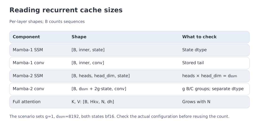 A recurrent serving passport: layer types, SSM state, convolution state, channel counts, state width, and dtype.
15. A current architecture passport
| Family | Sequence mechanism | Published contract | Context | Evidence |
|---|---|---|---|---|
| Mamba | selective SSM | attention-free backbone in the original work | up to 1M in author experiments | paper + code |
| Mamba-2 | SSD/SSM | recurrence and chunked matrix form | checkpoint-dependent | paper + code |
| Jamba | Mamba + attention + MoE | interleaved hybrid | up to 256K | paper/release |
| Falcon-H1 | Mamba-2 ∥ attention | parallel hybrid, 0.5B–34B | up to 256K | technical report |
| Qwen3.5-35B-A3B | 3 Gated DeltaNet : 1 full attention | 40 layers, 35B/3B, MoE | 262K native, ~1.01M extension | official card/config |
| Kimi K3 | 69 KDA + 24 Gated MLA | AttnRes is separate, 2.8T/104B | 1M | report/repository |
| Nemotron 3 Super | Mamba–Attention + LatentMoE + MTP | 120B/12B | up to 1M | official report |
| Nemotron 3 Ultra | Mamba–Attention + LatentMoE + MTP | 550B/55B | up to 1M | official report |
| MiniMax M2 | full attention | not a Lightning continuation | about 196K in open config | official note/config |
| MiniMax M3 | sparse attention | MSA, not fixed recurrent state | 1M report setting | paper/developer result |
| Mamba-3 | expressive recurrent SSM | complex/data-dependent state, MIMO | research setting | paper |
| SISA | SSM-derived term inside SDPA | retains the KV cache | research setting | paper |
The evidence column is part of the architecture description. For a closed model or incomplete report, “not disclosed” is more accurate than inferring an internal mechanism from a context-window number.
16. Audio, video, and other long streams
Recurrent carriers are attractive when a modality creates many sequential time steps: audio, video, sensor logs, genomics, or long agent trajectories. Fixed state lets the model keep processing without a cache that grows linearly with elapsed time.
Those modalities are not necessarily uniform, and they may still need exact recall of a particular event. A single recurrent state makes arbitrary random access difficult. Systems can respond with occasional attention, external retrieval, hierarchical memories, event indexes, or parallel recurrent and addressable branches.
A multimodal serving passport should therefore state both the recurrent state size and the mechanism used to revisit individual past events.
19. Key takeaways
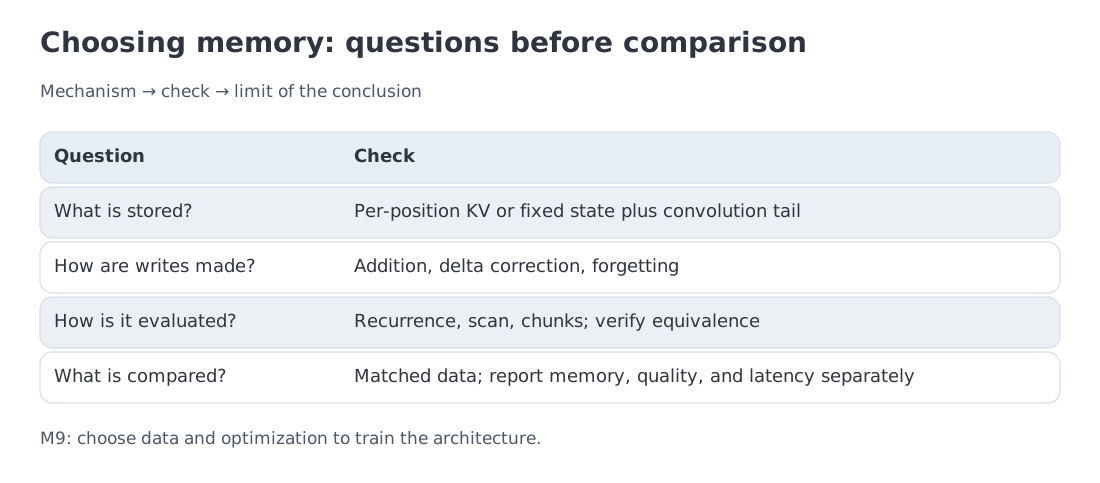 Exact discretization, selectivity, two cache states, SSD, delta rule, fixed-state bottlenecks, and hybrid layouts on one page.
- An SSM replaces an expanding list of past tokens with a fixed-size state.
- Mamba makes writing, reading, and forgetting input-dependent.
- A serving cache includes both SSM and causal-convolution state.
- SSD provides multiple execution forms for a structured class of SSMs.
- Delta rule edits an association; gating adds adaptive forgetting.
- Fixed state saves memory but creates an information bottleneck.
- Hybrids with full-attention layers retain length-dependent KV caches; fixed local windows give a different memory bound.
- Core-operator FLOPs are not end-to-end latency.
- Product-family names do not guarantee architectural continuity.
- A model should be read through layer types, cache shapes, state geometry, and source quality.
20. primary sources
Primary sources:
- Gu and Dao, Mamba
- Dao and Gu, Mamba-2 / State Space Duality
- Yang et al., DeltaNet
- Yang et al., Gated Delta Networks
- Lieber et al., Jamba
- Open Mamba implementation
- Qwen3.5-35B-A3B model card
- Kimi K3 repository and report
- Nemotron 3 Super
- Nemotron 3 Ultra
- Why MiniMax M2 uses full attention
- MiniMax M3
- Falcon-H1
- Mamba-3
- SISA
Next: Module 9 turns the architecture into a trained model: data selection, compute allocation, and optimization. Module 10 will then connect serving performance to memory bandwidth and roofline reasoning.
Sources rechecked on 11 October 2026. Memory figures are teaching scenarios; author-reported measurements retain their original conditions.