Module 7. Mixture of Experts
“Modern LLMs” course · Module 7 lecture · edition 2026.10.25
What this module is about. In M6, the feed-forward network accounted for most of the parameters in our example Transformer block. A Mixture of Experts (MoE) replaces that single network with a bank of separate FFNs, called experts. Each token uses only a few of them, allowing stored capacity to grow without evaluating the entire bank on every token.
A small learned network, the router, decides which experts to use. We will follow its scores through selection and the weighted output, then ask how to keep the workload balanced. Explicit counts for gpt-oss and DeepSeek-V3 connect the mechanism to parameter storage and communication. More elaborate routing designs build on this foundation on the reference route.
Prerequisites. Modules 1, 5, and 6 provide the useful background: total versus active parameters, attention geometry, and the parameter cost of a SwiGLU feed-forward network. All notation needed for the calculations is introduced again here.
Reading routes. To understand the mechanism, read §1, then §§4–10 while skipping the B09/B10 implementation details, and finish with §19 apart from the LatentMoE point. Use Q1–Q5 and Q7 in §17, then E1 and E3–E4 in §18. Q6 and E5 follow §11; E2 and E6 extend the reference and project routes. Follow one token and keep track of selection, mixture weights, and system cost. For the implementation pass, revisit §§6–7, work through §§12–14, and run the notebook. Use §§2–3, 11, and 15–16 as a reference for history, alternative routers, and model-specific contracts. M5 attention and M6 feed-forward blocks are the required background.
1. The bargain: capacity without activating the whole bank
A dense feed-forward network applies every one of its matrices to every token. If we enlarge that network, stored capacity and token-level arithmetic rise together. MoE changes the unit of conditional execution. A layer stores complete feed-forward experts. A small router scores them using the token's hidden vector, then selects the largest scores: top-k routing. The input to this decision is the vector representation, not the vocabulary ID.
This creates two related but non-interchangeable quantities:
- total parameters describe the full bank that the serving system must make available;
- active parameters describe the parameters charged under a stated per-token counting convention.
Neither quantity is a direct measurement of intelligence or latency. Total size does not uniquely determine knowledge, and active size omits communication, attention, the output head, memory traffic, and hardware utilization unless the convention explicitly includes them. It is nevertheless a useful first decomposition.
The range is already wide among documented open models. gpt-oss-120b publishes 117B total and 5.1B active parameters with 128 experts and top-4 routing. DeepSeek-V3 reports 671B/37B. Kimi K3 reaches 2.8T/104B while selecting 16 of 896 routed experts. Those headlines come from different architectures and sometimes different counting rules. A responsible comparison therefore asks what is common, what is routed, and which vocabulary matrices or auxiliary modules are included.
The compute bargain also creates a systems bill. The expert bank must be stored somewhere, route decisions must become efficient batches, and devices must exchange token representations. At large distributed scale, architecture and runtime must be designed together. Our task here is to understand their interaction and calculate the associated costs; implementing a distributed runtime is outside the course.
2. From local specialists to trillion-parameter sparse models
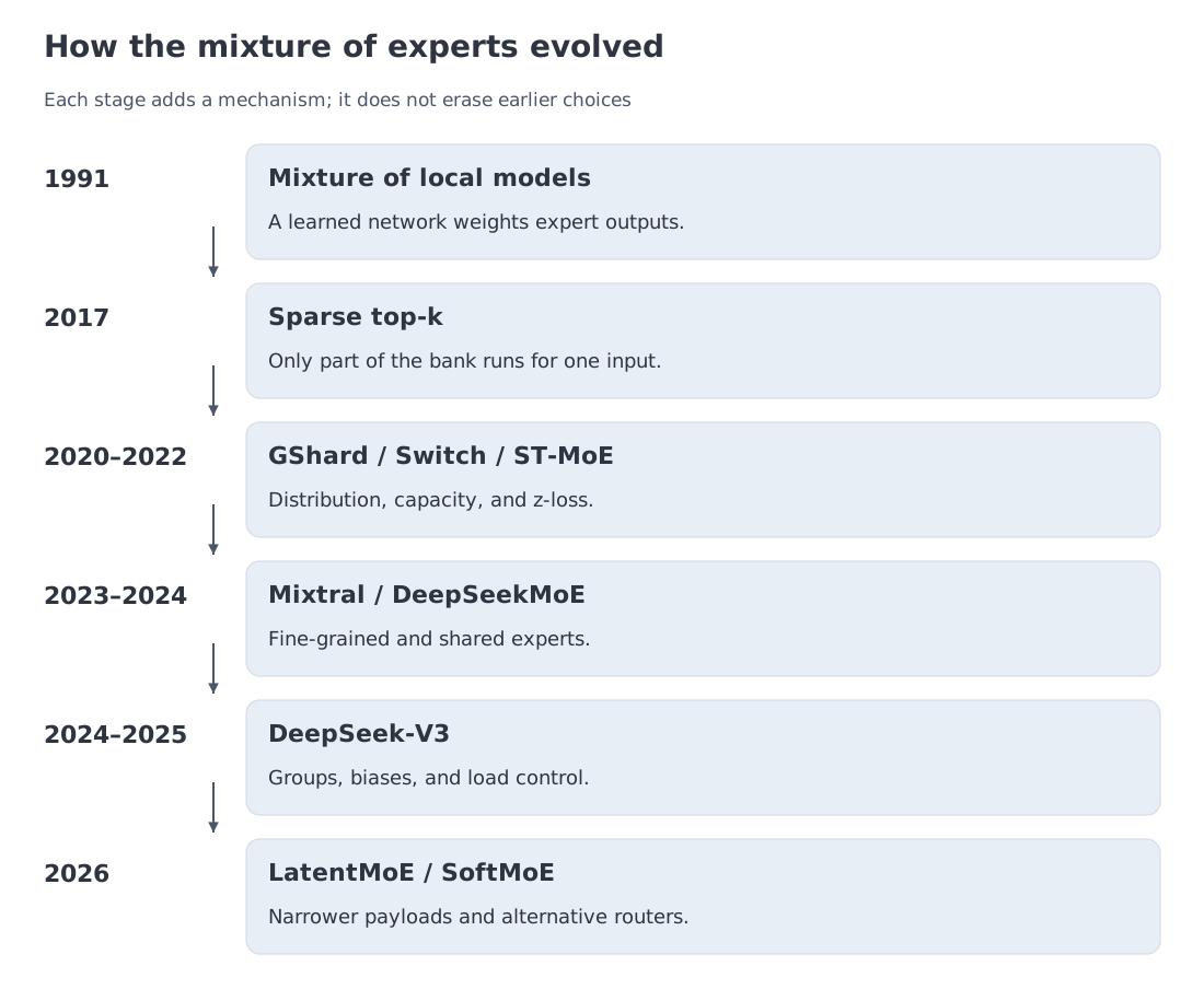 The evolution of MoE as a sequence of bottlenecks: learned gating, sparse top-k, expert parallelism and capacity, fine-grained/shared experts, auxiliary-loss-free balancing, and latent routed representations.
The statistical ancestor is the adaptive mixture of local experts introduced by Jacobs and Jordan. A gating network assigned examples to local predictors, allowing them to specialize. Modern MoE keeps that division of labor but changes both the scale and the computational shape.
Shazeer et al. brought sparsely gated experts to very large neural networks in 2017. Top-k routing made the parameter count enormous without evaluating every expert, but it also made expert collapse visible: a slightly favored expert receives more data, improves faster, and attracts still more tokens.
GShard and Switch Transformer turned sparse experts into a distributed Transformer component. Expert parallelism, capacity factors, all-to-all traffic, and token dropping became first-class concerns. Switch simplified routing to top-1; ST-MoE introduced router z-loss as one of its stabilization mechanisms.
Mixtral made top-2 MoE broadly inspectable in an open model. DeepSeekMoE then proposed finer expert segmentation and always-on shared experts. DeepSeek-V3 combined a large fine-grained bank with sigmoid scores, group preselection, and balancing biases updated outside the language-model objective.
Research through 11 October 2026 follows several different directions. LatentMoE compresses the routed representation and expert width. ReMoE and later differentiable methods modify top-k itself. Routing-free proposals remove a separate central router. The enduring idea is conditional expert compute; the exact routing and runtime contracts remain open design choices.
3. Three older ideas hiding inside modern MoE
A mixture model
The familiar form is
Sparse MoE makes most exactly zero through top-k selection. The experts are large dense FFNs, so selected work still maps well to matrix multiplication hardware.
Conditional computation
MoE is structured conditional execution. It differs from arbitrary weight sparsity because the active units are large blocks. A chosen expert can be evaluated by dense GEMM; the challenge is assembling enough tokens for each expert to make that GEMM efficient.
A distributed dispatcher
The router is also a scheduler. If one expert receives twice the load of its peers, the step may be limited by the device hosting that expert. A good probability model is therefore not enough: capacity, placement, networking, and queue behavior all matter.
These views explain why the module needs both equations and systems arithmetic. The mixture formula explains the output; conditional computation explains total versus active parameters; the dispatcher view explains load balancing and expert parallelism.
4. A typed contract for routing and parameter accounting
Separate two kinds of expert first. A routed expert runs only when selected; a shared expert runs for every token. Let the token vector be . The router's vector produces a logit . Applying the sigmoid gives an independent score:
A balancing controller can add an expert-wise selection bias . This is separate from a bias inside the linear projection. The selected index set is
A model may then normalize gates from the clean scores rather than the biased selection values:
The scale is an architecture setting: selected gates sum to . With shared experts, the expert branch returns
Both sums return vectors of width , ready to be added to the residual stream as in M6. A gate controls an output contribution; it need not be a calibrated probability of expertise. This sigmoid example is distinct from the selected-logit softmax used by gpt-oss in §14.
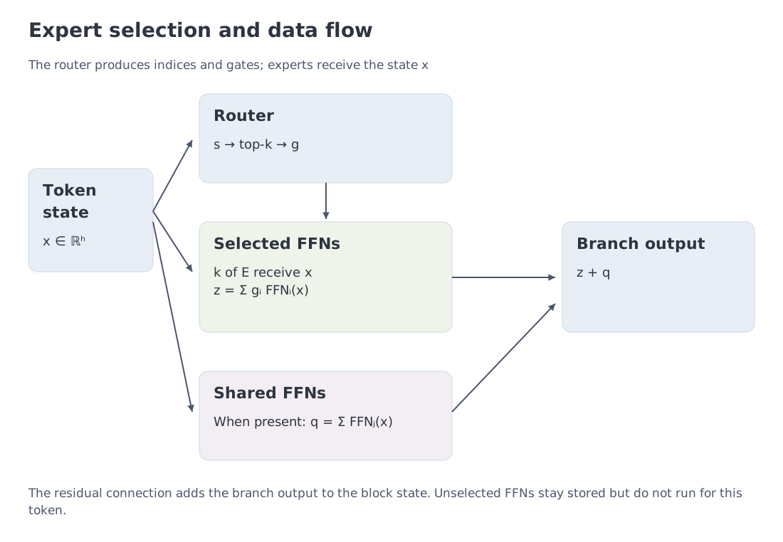 Residual state, router, top-k routed experts, always-on shared experts, and the distinction between the stored bank and one token's active path.
A SwiGLU expert with hidden width and expert intermediate width contains
matrix parameters. If all three projections have biases, the complete count is
No single total/active formula covers every model. A real count must state:
- how many layers are dense versus MoE;
- the number and width of routed and shared experts;
- whether embeddings are tied;
- which projections have biases;
- whether MTP or auxiliary modules are present;
- which full vocabulary matrices enter the active convention;
- the attention architecture and any extra normalization parameters.
For that reason, the numerical code uses a typed MoEModelSpec. It makes assumptions data rather than hiding them in algebra. In the gpt-oss examples, active parameters include one full vocabulary projection—the output head—but do not charge an indexed input embedding lookup as if every row had been multiplied.
5. Rebuilding both gpt-oss models from open code
The open implementation exposes details that a short configuration summary does not: QKV and output biases, router bias, expert biases, learned attention sinks, untied embeddings, and packed expert matrices.
Shared geometry for the two models:
- vocabulary size 201,088;
- hidden and expert intermediate width 2,880;
- 64 query heads, 8 KV heads, head width 64;
- two vocabulary matrices;
- biased attention projections, router, and experts.
gpt-oss-120b
With 36 layers, 128 experts, and top-4 routing, the complete reconstruction is:
| Component | Parameters |
|---|---|
| two vocabulary matrices | 1,158,266,880 |
| attention, including biases | 955,802,880 |
| all expert weights and biases | 114,701,598,720 |
| routers | 13,275,648 |
| normalization scales | 210,240 |
| learned sinks | 2,304 |
| Total | 116,829,156,672 |
Under the declared active convention:
and
The published 117B/5.1B values are appropriate rounded headlines. The course number is a reproducible count with its convention attached.
gpt-oss-20b
For 24 layers, 32 experts, and the same top-4:
Top-4 selects a much larger fraction of a 32-expert bank than of a 128-expert bank. The two models therefore have different sparsity factors despite sharing the same .
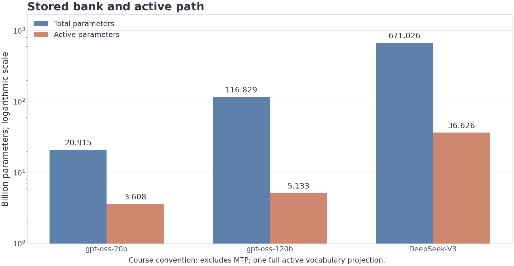 Total and active counts for the two gpt-oss models and the course reconstruction of DeepSeek-V3. A logarithmic plot does not erase differences in counting convention.
The rough estimate covers part of the weight-matmul arithmetic. It does not turn the 22.76 ratio into a latency multiplier: weight placement, expert batching, attention, and communication remain.
6. A numerical router trace
Take one token with router logits
[1.2, -0.3, 2.1, 0.4, 1.7, -1.0, 0.9, 2.5]
The sigmoid scores are
[0.7685, 0.4256, 0.8909, 0.5987,
 0.8455, 0.2689, 0.7109, 0.9241].
Top-4 selects experts
[7, 2, 4, 0]
with normalized gates
[0.2695, 0.2598, 0.2466, 0.2241].
Now give expert 3 a selection bias of . The selected set changes to
[3, 7, 2, 4].
The gate for expert 3 is still based on its clean score 0.5987, not on 0.9487. The gates become
[0.1837, 0.2835, 0.2733, 0.2594].
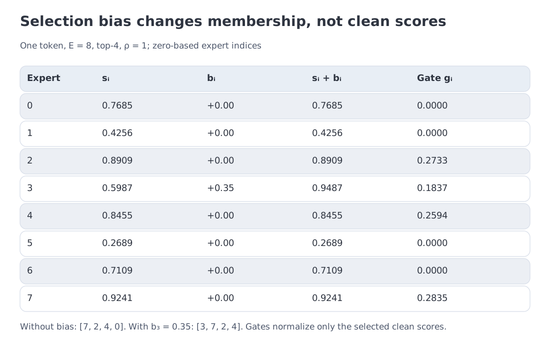 Clean scores, biased selection scores, selected experts, and gates. The balancing bias changes membership without entering the expert mixture weights.
DeepSeek-V3 adds a group stage. Its 256 routed experts are divided into eight groups; a token first retains four groups and then chooses eight experts from those groups. With balancing bias enabled, the group score is built from the two strongest adjusted scores in each group. Gates are then formed from clean scores and multiplied by the model's routed scaling factor.
This separation is broadly useful: a system can have one quantity for who is eligible and another for how much the selected output contributes.
Top-k indices are discrete. While membership stays fixed, selected mixture weights can carry gradients. With renormalized top-1, the single gate is identically one and this path cannot train the router. Gate normalization and other learning signals must therefore be inspected together; not every top-1 architecture renormalizes its selected gate to one.
Implementation and checks: B09
NumPy → PyTorch · B09 — Top-k MoE: expert selection and mixture weights
A selection bias may change expert choice while mixture weights still come from clean scores. NumPy makes the boundary explicit; PyTorch uses topk and gather.
import numpy as np
import torch
1. Explicit NumPy implementation
def numpy_topk_router_explicit(
    logits: np.ndarray,
    top_k: int,
    *,
    selection_bias: np.ndarray | None = None,
) -> tuple[np.ndarray, np.ndarray]:
    logits = np.asarray(logits, dtype=np.float64)
    if logits.ndim != 2 or not logits.size or not np.isfinite(logits).all():
        raise ValueError("expected non-empty finite logits[T,E]")
    if isinstance(top_k, (bool, np.bool_)) or not isinstance(top_k, (int, np.integer)) or not 1 <= top_k <= logits.shape[1]:
        raise ValueError("top_k must be an integer in [1,E]")
    log_scores = -np.logaddexp(0.0, -logits)
    clean = np.exp(log_scores)
    # Without bias, monotonic sigmoid permits ranking logits before saturation.
    selection = logits if selection_bias is None else clean + selection_bias
    if selection.shape != logits.shape or not np.isfinite(selection).all():
        raise ValueError("selection_bias must broadcast to [T,E] and be finite")
    indices = np.argsort(-selection, axis=-1, kind="stable")[:, :top_k]
    selected_log = np.take_along_axis(log_scores, indices, axis=-1)
    weights = np.exp(selected_log - selected_log.max(axis=-1, keepdims=True))
    weights = weights / weights.sum(axis=-1, keepdims=True)
    return indices, weights
Clean scores, selection priorities, and gates remain separate. Log-space normalization avoids 0/0 at very negative logits. Without bias, ranking logits avoids artificial ties caused by sigmoid saturation.
2. The same mathematics as explicit PyTorch operations
def torch_topk_router_explicit(
    logits: torch.Tensor,
    top_k: int,
    *,
    selection_bias: torch.Tensor | None = None,
) -> tuple[torch.Tensor, torch.Tensor]:
    if logits.ndim != 2 or not logits.numel() or not logits.is_floating_point() or not torch.isfinite(logits).all():
        raise ValueError("expected non-empty finite floating logits[T,E]")
    if isinstance(top_k, bool) or not isinstance(top_k, int) or not 1 <= top_k <= logits.shape[1]:
        raise ValueError("top_k must be an integer in [1,E]")
    z = logits.float() if logits.dtype in (torch.float16, torch.bfloat16) else logits
    log_scores = -torch.logaddexp(torch.zeros_like(z), -z)
    selection = z if selection_bias is None else log_scores.exp() + selection_bias
    if selection.shape != logits.shape or not torch.isfinite(selection).all():
        raise ValueError("selection_bias must broadcast to [T,E] and be finite")
    _, indices = torch.topk(selection, top_k, dim=-1)
    selected_log = log_scores.gather(-1, indices)
    weights = selected_log.softmax(dim=-1)
    return indices, weights
PyTorch uses log-sigmoid, topk, and gather, promoting FP16/BF16 to FP32. Gradients pass through selected gates, not discrete indices; topk tie order is unspecified. A renormalized top-1 gate is identically one and supplies no router gradient through this path.
| Aspect | NumPy | PyTorch |
|---|---|---|
| Clean scores | log-sigmoid → exp | log-sigmoid → exp |
| Selection | stable argsort | torch.topk |
| Selected weight | take_along_axis | gather |
| Bias | selection only | same contract |
| Ties | stable reference sort | ordering is not guaranteed |
Executable parity and edge-case check
logits_np = np.array([[2.1, -0.4, 0.8, 1.3], [0.2, 1.9, -1.1, 0.7]])
bias_np = np.array([0.0, 0.08, -0.03, 0.02])
i_np, w_np = numpy_topk_router_explicit(logits_np, 2, selection_bias=bias_np)
i_t, w_t = torch_topk_router_explicit(torch.tensor(logits_np), 2, selection_bias=torch.tensor(bias_np))
np.testing.assert_array_equal(i_np, i_t.numpy())
np.testing.assert_allclose(w_np, w_t.numpy())
extreme = np.array([[-1002., -1000., -1001., -1003.]])
with np.errstate(over="raise", invalid="raise", divide="raise"):
    ei, ew = numpy_topk_router_explicit(extreme, 2)
ti, tw = torch_topk_router_explicit(torch.tensor(extreme), 2)
np.testing.assert_array_equal(ei, [[1, 2]])
np.testing.assert_array_equal(ei, ti.numpy())
np.testing.assert_allclose(ew, tw.numpy(), rtol=1e-12, atol=1e-12)
z = torch.tensor(logits_np, requires_grad=True)
assert torch.autograd.gradcheck(lambda x: torch_topk_router_explicit(x, 2)[1], (z,))
one = torch_topk_router_explicit(z, 1)[1]
np.testing.assert_allclose(torch.autograd.grad(one.sum(), z)[0].numpy(), 0., atol=1e-12)
print("B09 routing, extreme logits, and selected-gate gradients: PASS")
Complete executable file: m07_moe_bridges.py
Tie-breaking contract: PyTorch topk.
7. Load balancing without conflating three mechanisms
A router can collapse through positive feedback. An early favorite receives more examples, learns faster, and becomes an even stronger favorite. Different mechanisms address different parts of that loop.
Auxiliary load-balancing loss
Take a batch of tokens and experts. The router assigns a softmax probability to expert for token . For top-1 routing, let be the fraction of tokens actually sent to that expert, and let be its mean probability before selection. These measure different objects: hard assignments and the router's continuous scores.
The Switch auxiliary term, before its external coefficient, is
If both distributions are uniform, each product is ; summing terms and multiplying by gives 1. During differentiation, the discrete assignments in are treated as fixed. Gradients pass through , providing a learning signal that reflects the observed load.
Training adds to the language-model objective. The coefficient sets the strength of this competing preference. In the notebook's top-k generalization, an expert receives assignments out of , so we define . The assignment fractions still sum to one; this normalization must be stated when comparing implementations.
Router z-loss
ST-MoE uses
where is the router logit for token and expert . Squaring happens before averaging across tokens. This penalizes each token's log-partition value, rather than bounding every logit individually. A separate coefficient sets its weight in the training loss; controlling numerical scale does not by itself balance expert assignments.
Auxiliary-loss-free balancing
An expert-wise bias is added before top-k and updated from recent loads outside backpropagation. The main rule in the paper is
Here counts assignments, is the expert average, and is the step size. An overloaded expert loses priority; an underused one gains it. This controller contributes no auxiliary gradient of its own, although changing assignments changes which experts learn from each token.
DeepSeek-V3 combines this batch-level controller with a small sequence-wise auxiliary loss to prevent extreme imbalance within an individual sequence. Auxiliary-loss-free balancing is the name of one mechanism, not a claim that the entire model has no auxiliary losses (report, §2.1.2).
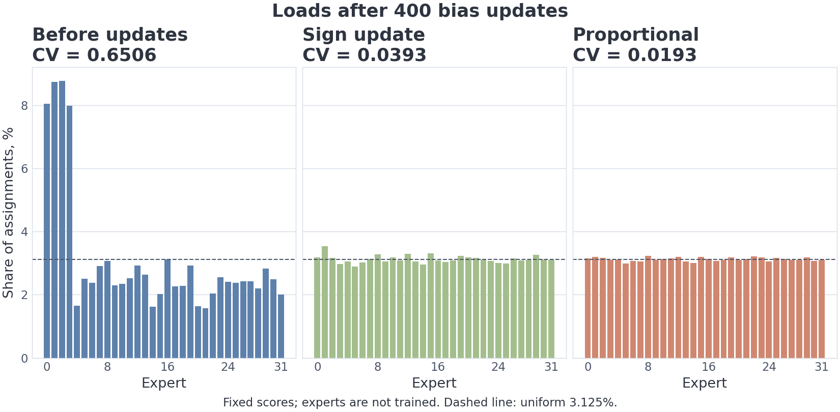 The paper-style sign update and a proportional teaching controller applied to the same deterministic score population.
We measure imbalance by the coefficient of variation, ; equal loads give zero. This experiment freezes router scores and updates only the biases, without training experts. It starts at CV 0.6506. After 400 updates:
- the sign rule with step 0.001 reaches 0.0393;
- the proportional teaching controller with rate 0.15 reaches 0.0193.
The smoother curve is not presented as the exact DeepSeek algorithm. It is an interpretable control-law experiment; the paper also analyzes a proportional variant in a separate setting.
An expert buffer has a separate limit. For tokens, assignments per token, and experts, the average is . A capacity factor allocates
slots per expert. The notebook accepts assignments in token order (FIFO), so earlier tokens can receive preferential treatment. Surviving gates are renormalized by course convention. Production implementations may reroute, allocate larger buffers, drop without renormalization, or use dropless grouped GEMM.
A token that loses every routed assignment does not vanish. Its routed branch is zero in that layer; any shared experts and the residual path continue.
8. Fine-grained experts and always-on shared capacity
Suppose an architecture replaces a small number of wide experts with a larger number of narrower ones while increasing proportionally. The active expert arithmetic can remain of similar order, while the router gains more ways to combine sub-blocks.
For a controlled example, replace 8 experts of width with 32 of width , and change top-2 to top-8. Expert matrix storage and active matrix arithmetic stay constant because and . The number of possible subsets rises from 28 to , while routing and communication costs may rise.
Another illustrative pair of bank sizes is
The latter 8/top-2 versus 128/top-4 comparison has no matched-budget claim. These numbers count unordered subsets, not learned skills. Continuous gate weights, correlated routing, and group constraints matter. For DeepSeek-V3, is only an unconstrained upper bound because group preselection rules out many subsets.
A shared expert follows a different path: it runs for every token. DeepSeekMoE motivates shared capacity as a place for common information and a way to reduce redundancy across routed experts. That motivation does not identify the content of one trained shared expert. Claims such as “this expert stores grammar” need intervention evidence, not just architecture diagrams.
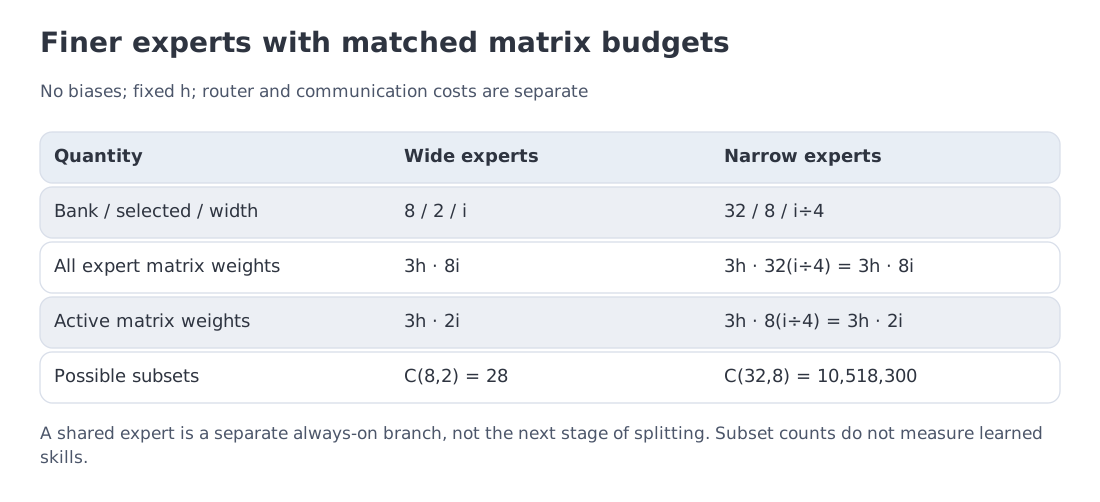 Coarse and fine-grained expert banks. More possible routing patterns increase flexibility, but the combinatorial count is not a semantic inventory.
DeepSeek-V3 reconstruction
Under the course's explicit convention:
These are consistent with the published 671B/37B headline. The Hugging Face package is about 685B when the 14B MTP module is included. A model passport should keep the main model, auxiliary modules, and active convention separate.
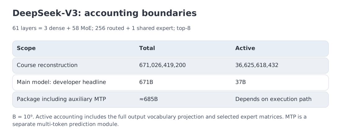 DeepSeek-V3: three dense layers, 58 MoE layers, 256 routed plus one shared expert, top-8, MLA, and a separately reported MTP module.
9. What expert specialization evidence can actually support
Routing statistics are easy to collect; semantic conclusions are harder.
Reliable observables include:
- expert frequencies by layer, language, or domain;
- co-activation matrices;
- changes after ablating or replacing an expert;
- router sensitivity to syntactic and semantic features;
- stability of a routing pattern across corpora.
A useful interpretation ladder is:
- routing preference: which inputs select an expert more often;
- functional effect: what changes under intervention;
- semantic label: a human summary that may be incomplete.
Experts often align with narrower operations or linguistic patterns rather than clean topics such as “mathematics” or “Chinese.” Several experts may be partly substitutable. The role of a shared expert can change across depth.
Supervised fine-tuning (SFT) updates model weights using training examples; M13 develops that process. To study its effect on experts, compare routing preferences and intervention results before and after the update. Evaluate language quality on held-out data as a separate measurement: a shift in expert frequency alone does not determine whether a language improved or degraded.
Serving systems care about a different pattern: hot experts under the actual product workload. Training-time balance does not guarantee balanced traffic after deployment. Per-expert utilization therefore belongs in production telemetry.
10. Inference: the expert bank, all-to-all, and batch union
The full bank must be available to the system, but it need not reside on one GPU or be replicated everywhere. Options include expert parallelism, CPU or NVMe tiers, weight streaming, hot-expert replication, and sharded caches.
Expert parallelism
Expert parallelism (EP) assigns experts to devices. Dispatch packs and sends their token vectors; combine returns and sums their outputs. An all-to-all exchange allows each device to send to every other, while grouped GEMM executes multiple expert matrix multiplications together.
Suppose every assignment moves a full vector of width and returns one of the same size, with bytes per coordinate. For one layer and the entire -token batch, the logical round-trip payload is
bytes. With , , , and bf16 (), this is 448 MiB across the batch, not per device. Actual network traffic can be lower because of local routes or destination-level aggregation, or higher because of padding and protocol overhead. This is assignment payload, not a universal network lower bound.
How many experts does a batch touch?
Under independent uniform routing, the expected fraction of experts touched by tokens is
For 128/top-4 and 256/top-8, is the same, so the theoretical curve is the same: at 64 tokens, the expected touched fraction is about 86.9%.
For Kimi K3's 896/top-16 routed bank:
- 16 tokens touch about 25.0% in expectation;
- 64 tokens touch about 68.4%.
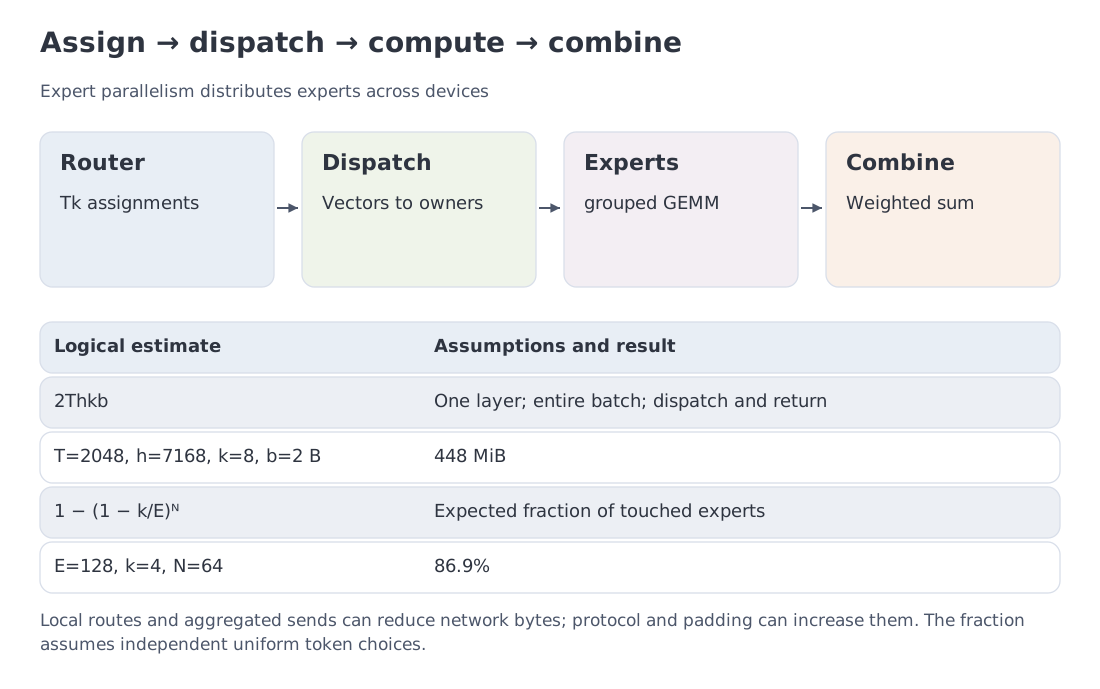 Dispatch, all-to-all, grouped expert computation, and return. The batch-union formula is shown with its independence and uniformity assumptions.
Actual routes can be correlated and skewed, and shared experts are always active. Group restrictions alone do not invalidate the law if each expert still has marginal selection probability and token choices remain independent. The formula is a baseline against which telemetry can be compared.
To assess expert offloading, measure popularity skew, temporal reuse, prefetching, and transport latency for the workload. A batch may need many more than the experts selected by one isolated token; useful prefetching must deliver their weights before the corresponding computation needs them.
11. LatentMoE and alternatives to fixed discrete top-k
LatentMoE keeps a discrete expert bank but reduces the width of the routed path. A hidden state of width is projected into a latent vector of width :
Dispatch, expert FFNs, and combination operate in that latent space. The result is projected back:
The router can still consume the original hidden representation and choose top-k experts. The two shared projections add matrix parameters. NVIDIA's shared experts, when present, stay in the original hidden width; the equation describes only the routed branch. Halving routed width therefore does not halve the whole model.
Kimi K3 uses hidden width 7168 and latent expert width 3584, giving a twofold idealized reduction in routed activation width. It retains 896 routed experts, top-16, and two shared experts. NVIDIA uses LatentMoE in Nemotron 3 Super and Ultra.
Several other branches change routing more directly:
| Method | Routing mechanism | Adaptive active count | Original evaluation domain |
|---|---|---|---|
| Soft MoE (2023) | soft token-to-slot and slot-to-token mixtures | fixed slot layout | vision Transformers |
| ReMoE | differentiable ReLU routing | effective dynamic sparsity | language models |
| SoftMoE (2026) | differentiable truncated soft top-k | yes, under a global budget | LLMs |
| Routing-Free MoE | removes a separate central router | method-dependent | research models |
These methods do not form one simple succession. They trade off differentiability, predictable kernel shapes, load balance, and adaptive compute.
12. Level-one code: policies should be visible
The educational implementation is intentionally small enough to inspect. It makes four choices explicit:
- selection scores and clean gate scores are separate;
- ties have a deterministic lower-index rule;
- capacity overflow is not silent;
- parameter counting is driven by a typed architecture specification.
This kernel exposes the order of operations in z-loss. B09 already gives the router; the notebook adds capacity, SwiGLU experts, and the shared branch.
from typing import Any
import numpy as np

def _finite_array(name: str, value: Any, *, ndim: int | None = None) -> np.ndarray:
    """Return ``value`` as a finite float64 array with an optional rank contract."""

    array = np.asarray(value, dtype=np.float64)
    if ndim is not None and array.ndim != ndim:
        raise ValueError(f"{name} must have rank {ndim}; got shape {array.shape}")
    if array.size == 0:
        raise ValueError(f"{name} must be non-empty")
    if not np.all(np.isfinite(array)):
        raise ValueError(f"{name} must contain only finite values")
    return array

def router_z_loss(logits: Any) -> float:
    """Compute the ST-MoE router z-loss ``mean(logsumexp(logits)^2)``."""

    raw = _finite_array("logits", logits)
    if raw.ndim != 2:
        raise ValueError("logits must have shape [T,E]")
    maximum = np.max(raw, axis=1, keepdims=True)
    log_partition = maximum[:, 0] + np.log(np.exp(raw - maximum).sum(axis=1))
    return float(np.mean(log_partition**2))
Implementation and checks: B10
NumPy → PyTorch · B10 — MoE dispatch and combine
Use hidden [T,D], indices and gates [T,K], and expert weights [E,D,F] and [E,F,D]. Indices are integers from 0 through E−1; repeated assignments are allowed and their contributions add. Floating arrays are finite with compatible dtypes; PyTorch tensors share a device. The minimal bridge validates indices before exposing dispatch and combination, without a capacity limit.
import numpy as np
import torch
1. Explicit NumPy implementation
def numpy_expert_dispatch_explicit(
    hidden: np.ndarray,
    expert_indices: np.ndarray,
    gates: np.ndarray,
    w_in: np.ndarray,
    w_out: np.ndarray,
) -> np.ndarray:
    if expert_indices.ndim != 2 or expert_indices.shape != gates.shape or expert_indices.shape[0] != hidden.shape[0]:
        raise ValueError("indices and gates must have matching shape [T,K]")
    if not np.issubdtype(expert_indices.dtype, np.integer):
        raise ValueError("expert indices must be integers")
    if np.any(expert_indices < 0) or np.any(expert_indices >= w_in.shape[0]):
        raise ValueError("expert index out of range")
    output = np.zeros_like(hidden)
    for token in range(hidden.shape[0]):
        for slot in range(expert_indices.shape[1]):
            expert = int(expert_indices[token, slot])
            mid = np.tanh(hidden[token] @ w_in[expert])
            output[token] += gates[token, slot] * (mid @ w_out[expert])
    return output
Two-matrix tanh experts keep this bridge focused on dispatch/combine. The token/slot loop adds each weighted expert output. The main notebook layer separately implements SwiGLU.
2. The same mathematics as explicit PyTorch operations
def torch_expert_dispatch_explicit(
    hidden: torch.Tensor,
    expert_indices: torch.Tensor,
    gates: torch.Tensor,
    w_in: torch.Tensor,
    w_out: torch.Tensor,
) -> torch.Tensor:
    if expert_indices.ndim != 2 or expert_indices.shape != gates.shape or expert_indices.shape[0] != hidden.shape[0]:
        raise ValueError("indices and gates must have matching shape [T,K]")
    if expert_indices.dtype not in (torch.int8, torch.int16, torch.int32, torch.int64, torch.uint8):
        raise ValueError("expert indices must be integers")
    if torch.any(expert_indices < 0) or torch.any(expert_indices >= w_in.shape[0]):
        raise ValueError("expert index out of range")
    output = torch.zeros_like(hidden)
    for expert in range(w_in.shape[0]):
        token_ids, slots = torch.where(expert_indices == expert)
        if token_ids.numel() == 0:
            continue
        mid = torch.tanh(hidden[token_ids] @ w_in[expert])
        expert_out = (mid @ w_out[expert]) * gates[token_ids, slots, None]
        output.index_add_(0, token_ids, expert_out)
    return output
PyTorch changes the execution order: assignments are batched per expert, then results are returned to tokens with index_add_.
| Aspect | NumPy | PyTorch |
|---|---|---|
| Order | token → slot | expert → assigned tokens |
| Expert batch | none | indexed hidden[token_ids] |
| Combine | output[token] += ... | output.index_add_ |
| Autograd | none | through expert matmul and combine |
| CUDA determinism | CPU reference | index_add_ may depend on atomic-add ordering |
Executable parity and edge-case check
rng = np.random.default_rng(10)
x_np = rng.standard_normal((6, 4))
idx_np = np.array([[0,1],[1,2],[2,0],[0,2],[1,0],[2,1]])
gates_np = np.full((6,2), 0.5)
w1_np = rng.standard_normal((3,4,5)); w2_np = rng.standard_normal((3,5,4))
np_out = numpy_expert_dispatch_explicit(x_np, idx_np, gates_np, w1_np, w2_np)
t_out = torch_expert_dispatch_explicit(torch.tensor(x_np), torch.tensor(idx_np), torch.tensor(gates_np), torch.tensor(w1_np), torch.tensor(w2_np))
np.testing.assert_allclose(np_out, t_out.numpy(), rtol=1e-10, atol=1e-10)
args = [torch.tensor(x_np, requires_grad=True), torch.tensor(idx_np),
        torch.tensor(gates_np, requires_grad=True), torch.tensor(w1_np, requires_grad=True),
        torch.tensor(w2_np, requires_grad=True)]
assert torch.autograd.gradcheck(
    lambda x, g, a, b: torch_expert_dispatch_explicit(x, args[1], g, a, b),
    (args[0], args[2], args[3], args[4]))
for invalid in (-1, w1_np.shape[0], .5, np.nan, True):
    bad = np.full(idx_np.shape, invalid)
    for dispatch, values in (
        (numpy_expert_dispatch_explicit, (x_np,bad,gates_np,w1_np,w2_np)),
        (torch_expert_dispatch_explicit, tuple(torch.tensor(a) for a in (x_np,bad,gates_np,w1_np,w2_np))),
    ):
        try: dispatch(*values)
        except ValueError: pass
        else: raise AssertionError("invalid expert index accepted")
duplicate = np.zeros_like(idx_np)
expected = idx_np.shape[1] * (np.tanh(x_np @ w1_np[0]) @ w2_np[0])
actual = numpy_expert_dispatch_explicit(x_np,duplicate,np.ones_like(gates_np),w1_np,w2_np)
np.testing.assert_allclose(actual,expected)
actual_t = torch_expert_dispatch_explicit(torch.tensor(x_np),torch.tensor(duplicate),
    torch.ones_like(torch.tensor(gates_np)),torch.tensor(w1_np),torch.tensor(w2_np))
np.testing.assert_allclose(actual_t.numpy(),expected)
print("B10 values, gradients, repeated assignments, and invalid indices: PASS")
Complete executable file: m07_moe_bridges.py
Accumulation contract: PyTorch index_add_.
14. Reading the gpt-oss implementation
The open reference code makes its routing contract unusually clear.
MLPBlock.gate has a weight matrix and a bias, takes top-k router logits, and applies softmax over the selected logits. That is not the sigmoid-plus-selection-bias contract used by DeepSeek-V3.
The expert implementation stores packed gate/up weights, corresponding biases, down weights, and down biases. The linear-layer biases contribute 40,105,728 parameters to the 120b model. In the original implementation, the packed gate and up columns alternate; a split into two contiguous halves would change the activation.
The original reference path gathers the selected expert tensors and uses einsum for both expert projections and the weighted sum. Bridge B10 uses a different, deliberately transparent execution order: a loop over experts and indexed addition. Serving implementations can instead use fused dispatch and grouped matrix multiplications across devices; the routing mathematics must still agree.
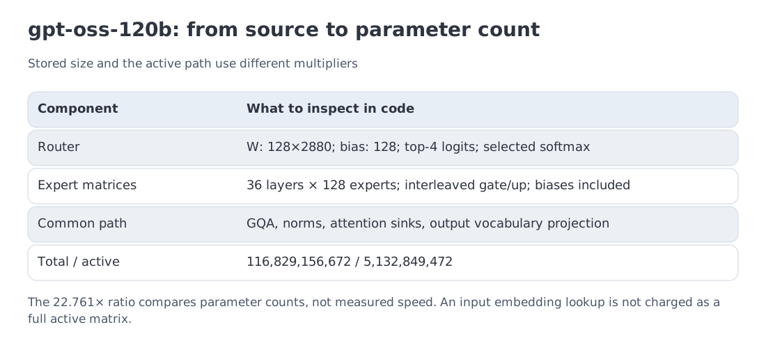 The gpt-oss-120b contract recovered from code: biased router, 128 routed experts, top-4, packed expert tensors, and an explicit active-count convention.
The general reading lesson is portable: inspect the score function, selection bias, gate normalization, shared capacity, expert tensor shapes, overflow policy, and distributed execution path. “MoE” alone specifies none of them.
15. A source-aware snapshot of current MoE architectures
The table is dated 11 October 2026 and records evidence rather than ranking models.
| Model | Total / active | Expert contract | Routing or related design | Evidence |
|---|---|---|---|---|
| gpt-oss-120b | 117B / 5.1B | 128 routed, top-4, no shared expert | softmax over selected logits | official announcement, config, and code |
| DeepSeek-V3 | 671B / 37B | 256 routed + 1 shared, top-8 | sigmoid, group preselection, loss-free bias | technical report and inference code |
| Qwen3.5-35B-A3B | 35B / 3B | 256 routed + 1 shared, top-8 | hybrid DeltaNet/attention, MTP | official model card and config |
| Kimi K3 | 2.8T / 104B | 896 routed + 2 shared, top-16 | Stable LatentMoE, latent width 3584 | official report and weights |
| Nemotron 3 Ultra | 550B / 55B | LatentMoE | hybrid Mamba–Attention, MTP, NVFP4 | official technical material |
| GLM-5 | 744B / 40B | 256 routed + 1 shared, top-8 | sigmoid/no-aux routing; DSA in attention | official model card and config |
| DeepSeek-V4 Pro / Flash | 1.6T / 49B; 284B / 13B | report-specific MoE | hybrid attention and MoE | technical report |
The active ratios are not directly comparable performance predictors. Models differ in dense prefixes, attention, MTP, modality towers, output heads, and counting conventions.
Qwen3.5-35B-A3B is a useful configuration-reading example. Its language model has hidden width 2048, 40 layers, 256 routed experts, top-8 plus one shared expert, expert intermediate width 512, and an MTP layer. Its block pattern interleaves Gated DeltaNet and full attention. A separate sigmoid gate scales the shared expert output. The presence of MTP in the configuration does not mean that ordinary autoregressive decoding runs it on every step: active accounting must specify the execution path.
16. Multimodal MoE is not one architecture
Multimodality can meet sparse experts in several ways.
A unified residual stream may send text and visual tokens through one routed bank. That enables mixed functional specialization but can widen the expert union touched by a batch. Kimi K3 is a current documented example of a native multimodal MoE system.
Another architecture can reserve modality-specific experts, trading simpler specialization for more complex balance and placement. A third can keep a separate vision encoder and route only the projected visual tokens through the language backbone.
If every token still chooses experts, expert compute per token does not rise merely because the token is visual. What can rise is the number of distinct experts touched across the mixed batch and therefore communication diversity. A multimodal MoE must be evaluated with routing and all-to-all telemetry, not only a total/active headline.
19. Key takeaways
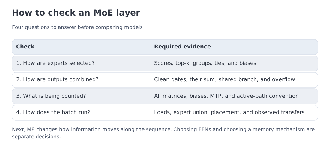 One-page map: declared total/active accounting, router and selection bias, load control, shared/fine-grained experts, expert parallelism, batch union, and LatentMoE.
- MoE grows stored capacity faster than per-token expert compute, but storage and communication remain.
- Total and active counts are meaningful only with a declared convention.
- A selection bias can alter top-k without becoming an expert mixture weight.
- Auxiliary-loss-free balancing removes a direct auxiliary gradient, not the effect of routing on training.
- Fine-grained banks create more routing flexibility; combinatorial subsets are not semantic skills.
- Shared experts reduce pressure to duplicate common computation, but their contents must be measured.
- Batch union can touch a large part of the bank; the uniform formula is a baseline.
- LatentMoE keeps discrete top-k while compressing the routed path.
- Current model tables should cite configs, reports, or code rather than inherit properties across families.
20. primary sources
Primary sources:
-
Jacobs et al., Adaptive Mixtures of Local Experts — paper
-
Shazeer et al., Outrageously Large Neural Networks — arXiv:1701.06538
-
GShard — arXiv:2006.16668
-
Switch Transformer — arXiv:2101.03961
-
ST-MoE — arXiv:2202.08906
-
DeepSeekMoE — arXiv:2401.06066
-
Auxiliary-Loss-Free Load Balancing — arXiv:2408.15664
-
DeepSeek-V3 — technical report and official repository
-
gpt-oss — official announcement and open implementation
-
LatentMoE — NVIDIA Research
-
Nemotron 3 Ultra — official page
-
Kimi K3 — official repository and report
-
Qwen3.5-35B-A3B — official model card
-
GLM-5 — official model card and config
-
Soft MoE — arXiv:2308.00951
-
ReMoE — arXiv:2412.14711
-
SoftMoE 2026 — arXiv:2606.17952
-
Routing-Free MoE — arXiv:2604.00801
-
DeepSeek-V4 — model card
Next: Module 8 changes the other large component of the block. Instead of routing among feed-forward experts, it asks whether sequence information must always move through attention, or whether recurrent state and state-space models can carry part of the load.
Landscape verified: 11 October 2026. Course reconstructions are separated from rounded developer headlines, and reported research results retain their original experimental scope.