Module 15. Reasoning Models and Test-Time Compute
What this module is about. The previous modules improved a model before deployment: pretraining built the base policy, supervised fine-tuning shaped its interface, and feedback-based learning changed which outputs it prefers. This module studies a different lever. Once the weights are fixed, a system can still spend more computation on a particular request—by extending one solution path, sampling several alternatives, checking them, or routing difficult prompts to a more expensive procedure.
These mechanisms are often grouped under test-time compute, but they buy different things. A longer trajectory deepens a single search. Parallel candidates widen the search distribution. A verifier turns candidate generation into selection. An adaptive controller decides which kind of work is worth paying for on each prompt.
We will treat quality and systems cost together. The module therefore follows reasoning tokens all the way down to decode latency, FLOP, KV memory, and concurrency. Numerical serving figures are explicit teaching scenarios, not performance claims about a particular vendor or accelerator.
Further study. Everything required for this module is developed here. The companion course RL for LLM goes deeper into RLVR, GRPO, verifier-driven training, and interactive environments, especially in Modules 9–10. Information Theory for ML provides a broader treatment of ensembles, uncertainty, and the value of additional observations.
Reading routes
First pass. Follow §§1–5, then read §§6–7 for the distinction between finding a correct candidate and selecting it. Continue through §§8–12 and §§15–17. The tables initially serve to show what changes as the budget grows. Use §18 to check that you can identify the generator, the verifier, and the cost of their work.
Second pass. Derive the probabilities in §§6–7, reproduce the accounting in §§10–12, and run §13 together with the notebook in §14. Work through §19 with particular attention to tie policies, independence, and the difference between a budget cap and actual consumption.
Reference pass. §§4 and 17 provide an API comparison checklist; §15 compares verification contracts. The API examples are dated observations, not a permanent model ranking.
The prerequisites are conditional probability, the KV-cache accounting in Module 10, and the SFT/RL distinction from Modules 13–14. RLVR means reinforcement learning with verifiable rewards, such as exact-answer checks or executable tests. Here a related checking signal will also guide inference while model weights stay fixed.
1. A second scaling axis
We need four terms before comparing policies. A trajectory is one sequence of intermediate actions ending in an answer. A candidate is the result of an attempt that can be compared with others. A verifier checks or scores it; a selector uses that evidence to choose an answer. In best-of-N, the system generates candidates and returns the highest-ranked one under a specified rule. “Best” refers to that rule, which may disagree with correctness.
A large language model is usually evaluated as though it had one chance: one prompt enters, one completion leaves. That convention hides an important design choice. We can also ask how well the same trained model performs when it is allowed to spend more computation on the instance in front of it.
There are three broad ways to spend that budget.
- Go deeper. Continue one trajectory, revise an intermediate step, run a longer plan, or interleave reasoning with tools.
- Go wider. Produce independent candidates, perhaps from one model or from several agents, and then aggregate or select.
- Allocate adaptively. Give easy inputs a short path and reserve expensive search for requests that appear difficult or uncertain.
All three need a decision rule. A long chain needs a stopping condition. A candidate pool needs a selector. An adaptive system needs a signal that says whether more work is likely to pay off.
This is why inference-time scaling is not merely “turning up intelligence.” It is an algorithm for allocating a finite resource. Snell et al. showed that the most effective allocation varied strongly with prompt difficulty. Under their experimental setup, compute-optimal routing used test-time computation more than four times as efficiently as a simple best-of-N baseline, and a smaller model could beat a model fourteen times larger on a subset of tasks under FLOP-matched evaluation. Those are study-specific results, but the underlying lesson is general: the allocation policy is part of the method. Snell et al., 2024
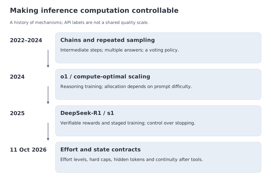 From the first public reasoning systems to controllable and adaptive inference contracts.
2. From longer traces to explicit controls
Chain-of-thought prompting, self-consistency, and generate-and-test workflows predate the current generation of reasoning models. The 2024–2026 shift was more specific: model training and product interfaces began to treat inference computation as a resource that could be deliberately scaled.
OpenAI's September 2024 o1 announcement described performance improving along two axes: more reinforcement-learning compute during training and more time spent reasoning at test time. The public article did not disclose a full recipe, but it made inference-time scaling a first-class claim rather than a prompting trick. OpenAI, 2024
DeepSeek-R1 supplied a much more inspectable training story in January 2025. R1-Zero used large-scale reinforcement learning on verifiable signals without a preliminary supervised phase. The model developed longer solutions, self-checking behavior, and course corrections, while also suffering from readability and language-mixing problems. The full R1 pipeline then combined cold-start data, reasoning RL, rejection sampling, renewed SFT, and broader RL objectives. DeepSeek-R1, 2025
By 11 October 2026, inference controls had become a regular part of model APIs, but the contracts were not standardized:
- GPT-6.1 Sol supports
low,medium(the default),high,xhigh, andmaxeffort. It does not supportnoneorminimal. - Claude Opus 5.5 uses adaptive thinking. Manual
budget_tokensand disabling thinking are unavailable on this model; effort and the display of intermediate content remain separate controls. - Gemini 3.8 Flash through the Interactions API accepts
generation_config.thinking_levelvalues oflow,medium, orhigh, withmediumas the default. The field name belongs to this API surface. - Kimi K3 always reasons and accepts
low,high, andmaxthroughreasoning_effort; its documented default ismax. - Inkling was trained for controllable reasoning effort according to its developer. That release claim describes this model, not a standard shared by other APIs.
The labels are local to each API. A high setting does not imply a common token count, latency target, search algorithm, or billing rule. Documentation tells us what control surface exists; it rarely reveals the complete internal computation. OpenAI API · Anthropic · Gemini API · Kimi K3 · Inkling
The important historical change, then, is not that models began emitting intermediate text. It is that reasoning depth, search breadth, and routing became deployable system parameters.
3. Three older ideas hiding inside test-time compute
Modern reasoning systems recombine several classical patterns.
Anytime computation
An anytime algorithm returns a usable answer early and improves it while resources remain. Search, planning, and numerical optimization all have examples. A well-designed reasoning model should exhibit the same property: extra time should be optional, and the system should be able to stop with a coherent result.
A token cap alone does not create an anytime algorithm. A hard cutoff can leave an unfinished derivation or no final answer. A practical controller can retain the best verified candidate so far and return it when the budget expires. An incomplete new attempt then cannot erase an existing usable result.
Repeated stochastic search
If one attempt has a non-zero chance of success, independent restarts increase the chance that a successful path appears. This is the same intuition behind ensembles and randomized search. Yet a pool containing a correct answer is useful only if the system can identify it.
Generate and test
Program synthesis, theorem proving, and planning often separate proposal from validation. Generate a candidate; run a compiler, unit tests, a proof kernel, or a simulator; keep what passes. This arrangement is especially attractive when generation is uncertain but checking is cheap and exact.
The mapping is straightforward:
- sequential reasoning is a form of deeper search;
- multiple completions form a stochastic ensemble;
- a verifier supplies the acceptance or ranking rule;
- an adaptive controller is a meta-policy over those choices.
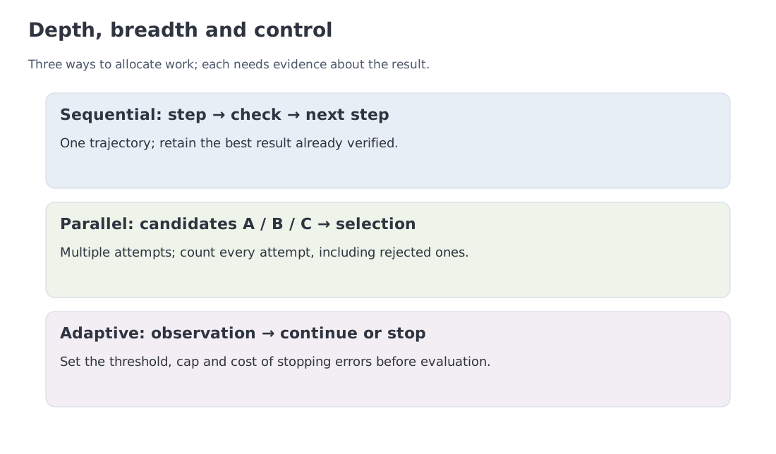 Three ways to spend inference compute: deepen one path, widen the candidate set, or route adaptively.
4. What counts as a reasoning model?
The phrase can easily be overinterpreted. A visible chain of text is not guaranteed to be a faithful transcript of internal computation, and a hidden chain is not automatically more rigorous. We will use a functional definition:
A reasoning model is trained or deployed so that additional computation before the final answer can be used productively.
That property has several separable dimensions.
Representation. Intermediate work may be exposed, hidden, summarized, placed in a dedicated message field, or represented by opaque signatures needed for continuity. A <think> token in a chat template establishes a format, not a capability guarantee.
Control. The user may specify a token target, select an effort level, enable an adaptive mode, or receive no direct control at all.
Topology. Increasing one model's effort and launching several workers are separate choices. A max setting does not specify the number of parallel candidates. Meta describes Muse Spark 1.1 as supporting planning and delegation in agent harnesses. When a chosen harness delegates work, its evaluation must count all workers' computation. This describes supported system behavior rather than establishing the model's internal architecture. Muse Spark 1.1
Accounting. Reasoning tokens can consume output limits and be billed even when only a summary is visible. Gemini reports thought-token usage separately in metadata while charging for the underlying generated thinking tokens. Gemini API
State across turns. Some APIs require the application to return complete assistant messages, thought signatures, or reasoning items after tool calls. Dropping those fields may discard useful state or violate the protocol.
A proper comparison therefore needs more than an effort label. It needs the depth of one trajectory, the number of parallel attempts, the selection rule, the visibility contract, and the accounting model.
5. What DeepSeek-R1 teaches us about training reasoning
DeepSeek-R1 is useful because its report separates an exploratory RL result from a deployable multi-stage system.
R1-Zero as a controlled experiment
The starting checkpoint is the pretrained DeepSeek-V3-Base. “Without preliminary SFT” describes the reasoning post-training stage; language knowledge and representations already exist. The experiment does not train a language model from scratch using rewards alone.
R1-Zero did not receive a supervised warm-up that taught it how a long solution should look. It was optimized with reinforcement learning on verifiable rewards and formatting constraints. During training, solutions became longer and exhibited behaviors such as checking previous work and trying another route.
The defensible conclusion is not that a language model acquired human cognition. It is narrower: a policy can discover token-level computational strategies when exploration is coupled to an informative, verifiable reward.
The experiment also exposed the cost of optimizing correctness in isolation. Outputs could be hard to read, switch languages, or use an inconvenient format. A useful assistant needs both problem-solving behavior and a stable human-facing interface.
The full R1 pipeline
The complete recipe adds several stages:
- a small cold-start SFT set for readable reasoning behavior;
- reasoning-focused reinforcement learning;
- collection of successful trajectories from the RL checkpoint, followed by SFT of DeepSeek-V3-Base on those trajectories and a broader data mixture;
- additional reinforcement learning for general helpfulness, safety, and instruction following.
This is a good antidote to the false choice between SFT and RL. Supervised data establish a usable format; RL explores under reward; selected trajectories become new data; broader post-training restores the full interaction contract.
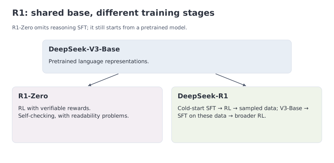 R1-Zero isolates the RL mechanism; DeepSeek-R1 combines it with cold-start data and broader post-training.
6. Parallel scaling, worked example A: voting can get worse first
Assume that one independent completion is correct with probability
When it is wrong, the answer is uniformly distributed across six distinct distractors. We draw completions and return the most frequent normalized answer.
The procedure is still underspecified. What happens when several answers share the top count? We compare two exact policies:
- tie means failure: the correct answer must be the unique mode;
- random top-mode selection: choose uniformly among all modes tied for first place.
A distractor is an incorrect answer option. A mode is the most frequent option. This is plurality voting: the winner need not receive more than half the votes. Let count occurrences of answer , with index reserved for the correct answer. Then and . Independence gives the multinomial probability
The factorial term counts the sequences that produce the same counts. For the strict policy, sum this mass over outcomes satisfying . For random tie-breaking, also include outcomes where the correct answer ties for first, weighted by when options share the lead.
For , a unique correct mode requires two or three correct draws. An independent check is therefore . At larger sample sizes, a unique mode can win without an absolute majority, so the full count vector matters.
Enumerating the multinomial outcomes gives:
| unique-mode success | random tie-breaking | |
|---|---|---|
| 1 | 0.400 | 0.400 |
| 3 | 0.352 | 0.472 |
| 5 | 0.509 | 0.596 |
| 9 | 0.671 | 0.737 |
| 17 | 0.857 | 0.889 |
At , a top-mode tie occurs with probability 0.48. Under the strict rule, three samples are worse than one. The result is not a paradox; it is a reminder that tie handling is part of the algorithm.
A reproducible self-consistency protocol must also define answer normalization. Are 0.5, 1/2, and 50% equivalent? Are algebraically equivalent expressions canonicalized? Are code outputs compared by text or by execution? Small implementation choices can dominate the apparent gain from extra sampling.
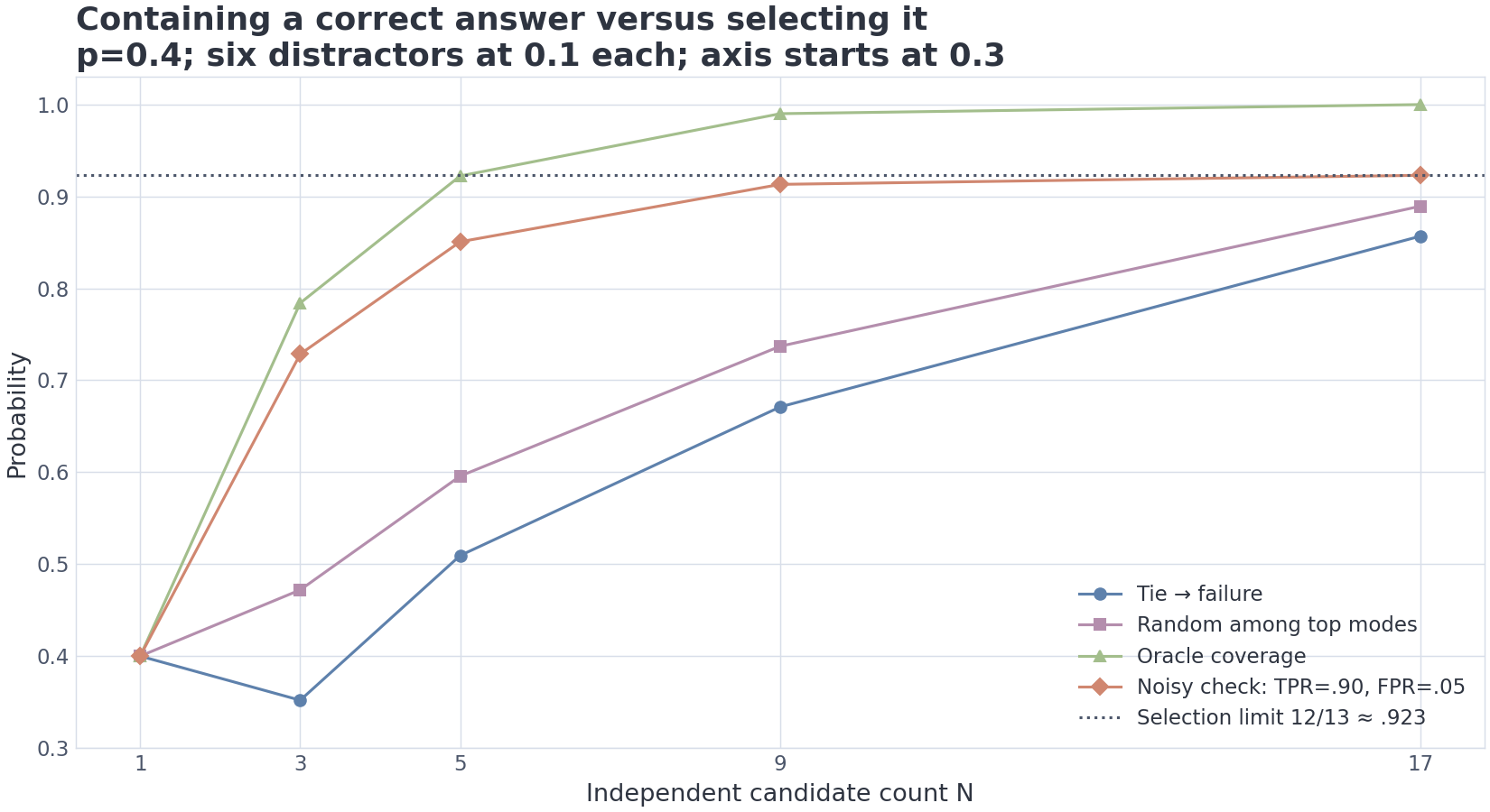 Exact voting policies, oracle coverage, and selection by a noisy verifier.
The Large Language Monkeys study showed that repeated sampling can improve coverage over very large ranges of sample count. In automatically verifiable domains, coverage can translate directly into solved tasks. Where selection relies on majority vote or imperfect reward models, the selector can plateau even while the generator continues to produce additional correct candidates. Brown et al., 2024
7. Worked example B: coverage is not selection accuracy
Voting uses frequency as a proxy for correctness. A verifier uses evidence about the candidate itself. Before modeling an imperfect verifier, we need an upper bound.
For independent attempts with success probability , the probability that at least one of candidates is correct is
With :
| oracle coverage | |
|---|---|
| 1 | 0.400 |
| 3 | 0.784 |
| 5 | 0.922 |
| 9 | 0.990 |
| 17 | 0.9998 |
This curve tells us what an oracle could recover. It says nothing about whether an actual ranking model will find the correct item.
Use an accept/reject verifier with true-positive rate (TPR) 0.90: it accepts a correct candidate with probability 0.90. Its false-positive rate (FPR) is 0.05: it accepts an incorrect candidate with probability 0.05. Checks are independent across candidates conditional on correctness. Select uniformly among accepted candidates; if none pass, select uniformly from the entire generated pool. This precise policy gives:
| noisy-verifier accuracy | |
|---|---|
| 1 | 0.400 |
| 3 | 0.728 |
| 5 | 0.851 |
| 9 | 0.913 |
| 17 | 0.923 |
The plateau is approximately 0.923, rather than the verifier's TPR of 0.90. To see why, define the probability of accepting an arbitrary candidate, , and the correctness rate among accepted candidates, :
For , the selection policy has the closed form
When at least one candidate is accepted, a uniform accepted candidate is correct with probability . If every candidate is rejected, a random rejected candidate is correct with probability . Weighting the two events yields the expression above. The boundary is read directly from the selection rule; if , nothing is ever accepted and .
Here and . A single candidate gives ; a large pool approaches . TPR is the probability of acceptance given correctness, whereas reverses that conditioning. Confusing them changes the predicted limit.
With constant rates and TPR > FPR, this model improves monotonically. A decline under more search needs an additional mechanism, such as selecting an extreme noisy score or actively finding candidates that exploit the verifier. The latter resembles reward hacking from Module 14.
Independence also needs care. Perfectly correlated errors give no coverage gain at all. Even independent attempts on each task do not justify substituting average task accuracy into the coverage formula. If half the tasks have and half have , the mean is 0.4, but three-attempt coverage is , not 0.784. Task difficulty is shared across attempts.
A sensible verification hierarchy is:
- a formal checker or deterministic executable rule;
- unit tests and explicit constraints;
- a specialized process or outcome model;
- a general LLM judge with a documented rubric;
- voting when no stronger signal is available.
An LLM judge should not replace a compiler or proof kernel merely because it is convenient.
8. Sequential scaling and budget forcing
Parallel inference restarts the search. Sequential inference gives one trajectory more room to evolve.
The s1 paper provides a clean demonstration. The authors curated 1,000 difficult, diverse, high-quality reasoning examples, fine-tuned Qwen2.5-32B-Instruct, and then controlled the length of its reasoning without another weight update. Their budget forcing procedure could:
- extend a trace by appending
Waitwhen the model attempted to finish; - shorten a trace by forcing the transition to the final answer.
Under the reported AIME 2024 setup, increasing the budget raised s1-32B from 50% to 57%. That is evidence for one model and evaluation protocol, not a law that every task improves with every extra token. Muennighoff et al., 2025
The intervention changes decoding while leaving weights fixed. Extra steps may let existing operations produce a new deduction or find a missed solution. They do not guarantee recovery of a missing fact; consulting a tool or an external source adds information through a separate mechanism.
Sequential compute can support several policies: continue the current derivation, insert explicit checks, revisit a branch point, alternate planning with tool execution, or stop early once evidence is sufficient. A mature system needs the last operation as much as the first. Scaling inference includes learning when not to continue.
9. Failure modes of longer reasoning
Extra tokens are useful only if they change the computation in a productive direction.
Overthinking. A model may reach the right answer quickly, then revise it into a wrong one. Empirical work has found non-monotonic relationships between chain length and accuracy, with shorter selections sometimes outperforming longer traces. The effect depends on the model, task, and selection protocol. Hassid et al., 2025; v2 2026
Length and correctness can correlate because harder tasks induce longer attempts. Comparing trajectories for the same prompt reduces that confounding, but still does not randomly assign length: the model partly chooses when to stop. To estimate the effect of additional budget, assign different budgets to the same prompts, repeat sampling, and hold the selection protocol fixed.
Redundant continuation. The model may restate the same hypothesis without creating new search state.
Error accumulation. An early false premise becomes part of the context and shapes every later step. Fluency can increase even as correctness falls.
Verifier exploitation. A search process can optimize whatever signal it sees. If the verifier rewards persuasive form, more search may find more persuasive errors.
The module notebook contains a deliberately synthetic illustration: difficult tasks improve with additional budget, while easy-task accuracy eventually declines. The curves demonstrate a possible mechanism; they are not measurements of a deployed model.
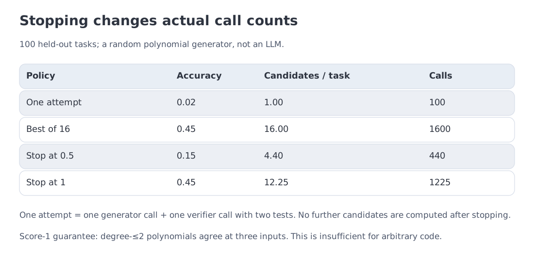 Executable polynomial search: actual calls and the cost of two stopping rules; the lab is explained in §14.
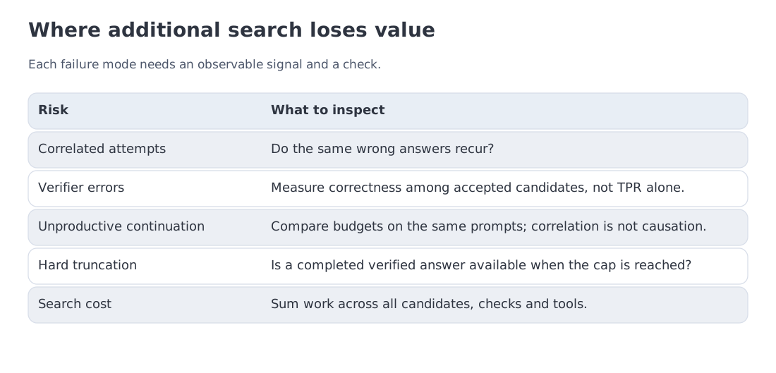 Observable search failures: correlated errors, weak verification, unproductive continuation, truncation, and cost.
10. Worked example C: an illustrative budget ladder
Provider effort labels do not map to a universal token count. To reason about systems cost, we therefore use an explicit course scenario rather than pretending to reconstruct an API.
Assumptions:
- a dense -parameter decoder;
- 209.4 sequential decode tokens per second, fixed as a course assumption;
- 512 tokens for a short baseline answer;
- illustrative budgets of 1K, 4K, 16K, and 64K generated tokens.
A common approximation to dense weight-matrix multiplication work is
and unbatched latency is
| illustrative tier | tokens | latency | weight-matmul FLOP estimate | vs. 512 tokens |
|---|---|---|---|---|
| short baseline | 512 | 2.45 s | 1× | |
| small | 1,000 | 4.78 s | 1.95× | |
| medium | 4,000 | 19.10 s | 7.81× | |
| large | 16,000 | 76.41 s | 31.25× | |
| very large | 64,000 | 305.64 s | 125× |
The factor of two counts a multiplication and an addition as two operations. The approximation is useful when weight-matrix multiplications dominate. It omits prompt processing, attention products over a growing context, tools, and verification. Architecture also affects which parameters do work; a MoE model's total stored parameter count cannot simply be substituted here.
Linear latency follows from the assumed constant 209.4-token/s rate. Actual decode throughput depends on context length, batching, and load, with queueing and prefill added to the request. A multi-candidate system must count discarded attempts as well. The calculation still conveys the scale of the tradeoff: five seconds and five minutes support different interactions.
Extending a trajectory from 2K to 8K tokens adds
Whether that is worthwhile cannot be decided from the cost equation. It requires an empirical quality curve on the target workload.
11. Worked example D: the KV cost of a thought
Consider a full-attention decoder that retains the entire history. In this model, each generated token adds K and V vectors in every attention layer.
Take an illustrative model with 32 layers, KV width 1,024 per layer, and bf16 storage. The KV bytes per token are
| reasoning length | KV per request |
|---|---|
| 512 | 0.0625 GiB |
| 1K | 0.122 GiB |
| 4K | 0.488 GiB |
| 16K | 1.953 GiB |
| 64K | 7.8125 GiB |
The table counts KV for generated tokens only, retaining the full history in all 32 layers. A prompt of tokens changes the total to KiB. With and , this is GiB rather than the continuation-only GiB. Windowed or hybrid architectures require per-layer accounting; shared prefixes can reduce physical storage across candidates.
The bounds below assume a zero-length input prefix and a teaching device with 80 GiB available capacity. That is an explicit capacity assumption, not a conversion of every marketed “80 GB” device.
The bf16 weights of an 8.03B model occupy about 14.96 GiB. If an 80 GiB device devoted every remaining byte to KV, the resulting upper bounds would be 1,040 concurrent 512-token requests, 532 at 1K, 133 at 4K, 33 at 16K, and only 8 at 64K.
These are not throughput forecasts. They omit activations, fragmentation, scheduler state, batching, and runtime reserve. Reserving 8 GiB lowers the 1K–64K figures to 467, 116, 29, and 7. The calculation still exposes the order of magnitude: moving from 512 to 64K tokens reduces a KV-limited concurrency bound by roughly 130×.
This is why the serving techniques from Module 10—paged allocation, KV quantization, offload, and tiered storage—become central for reasoning workloads rather than optional optimizations.
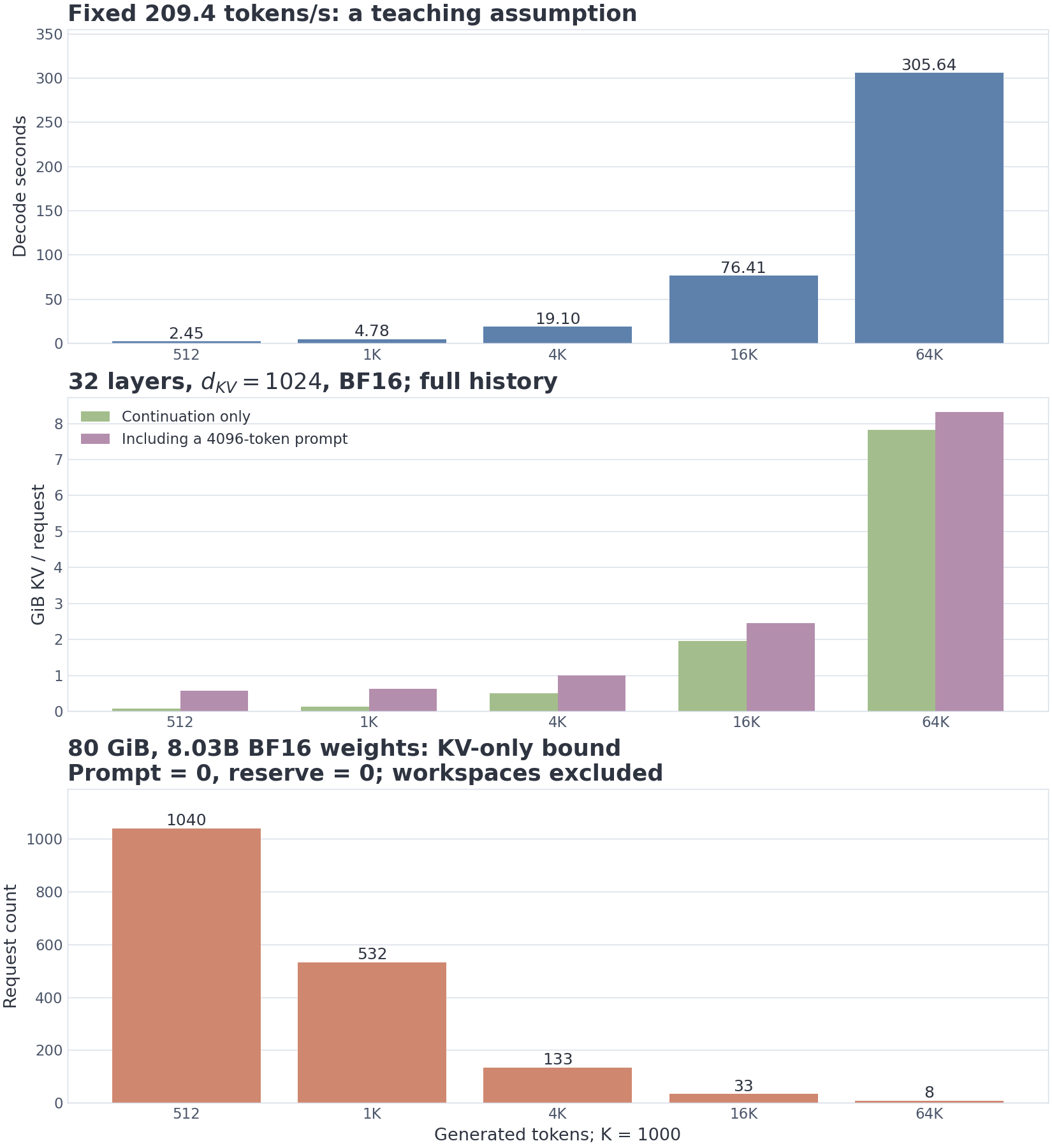 Assumed decode time, KV with and without a prompt, and a KV-only concurrency bound.
12. Worked example E: why adaptive allocation matters
Suppose a workload has three classes:
- 70% easy requests needing about 500 tokens;
- 20% medium requests needing about 4,000;
- 10% hard requests needing about 32,000.
Assume that every assigned budget is used in full and the router identifies each task class perfectly. A uniform maximum then costs 32,000 tokens per request, while the routed mixture costs
The ratio is
This calculation assumes a perfect router and full consumption of each assigned budget. A cap is not consumption: a model allowed 32,000 tokens may stop much earlier. A real comparison must measure actual tokens and quality, including the work needed to determine the route.
Possible routing signals include a cheap difficulty classifier, uncertainty after a short first pass, agreement between samples, a verifier threshold, or a signal from the environment such as passing tests.
The first notebook simulation precomputes all candidate labels and scores. It then asks how many entries a policy would inspect before reaching a score of 0.82 or exhausting 16 attempts. On this fixed mixture, it inspects 4.02 candidates on average and achieves 0.886 accuracy, versus 0.632 for one shot and 0.940 for selecting from all sixteen. These are policy comparisons on shared data; the vectorized simulation itself saves no generator calls.
A separate program-search lab then generates candidates inside the loop and actually stops further calls. §14 explains the experiment. Choose thresholds or budgets on a calibration split and evaluate the frozen policy on held-out tasks. Tuning them using the final test answers would bias the comparison.
Adaptive inference is therefore a classification-and-control problem under noise. A router can waste compute on easy inputs or prematurely stop hard ones. Its error costs belong in the evaluation.
13. Level-1 code: make selection and cost assumptions explicit
The first function computes oracle coverage. It deliberately does not claim to model a selector.
"""Coverage, noisy selection and scoped inference accounting."""
import math
from dataclasses import dataclass

def positive_count(value, name):
    if isinstance(value, bool) or not isinstance(value, int) or value <= 0:
        raise ValueError(name + " must be a positive integer")

def probability(value, name):
    if not math.isfinite(value) or not 0 <= value <= 1:
        raise ValueError(name + " must be finite and lie in [0, 1]")

def oracle_coverage(p_correct, n):
    """At least one success in n independent, identically distributed attempts."""
    positive_count(n, "n")
    probability(p_correct, "p_correct")
    if p_correct == 1:
        return 1.0
    return -math.expm1(n * math.log1p(-p_correct))

def noisy_selection(p, n, tpr, fpr):
    """Uniform accepted candidate; uniform pool fallback if none are accepted."""
    positive_count(n, "n")
    for name, value in (("p", p), ("tpr", tpr), ("fpr", fpr)):
        probability(value, name)
    acceptance = p*tpr + (1-p)*fpr
    if acceptance == 0 or n == 1:
        return p
    precision = p*tpr/acceptance
    if acceptance == 1:
        return precision
    log_survival = (n-1)*math.log1p(-acceptance)
    # A non-negative mixture avoids cancellation for tiny probabilities.
    return p*math.exp(log_survival) + precision*(-math.expm1(log_survival))

@dataclass(frozen=True)
class ReasoningCost:
    parameters: float = 8.03e9
    tokens_per_second: float = 209.4
    layers: int = 32
    kv_width: int = 1024
    bytes_per_element: int = 2

    def __post_init__(self):
        for name in ("parameters", "tokens_per_second"):
            value = getattr(self, name)
            if not math.isfinite(value) or value <= 0:
                raise ValueError(name + " must be finite and positive")
        for name in ("layers", "kv_width", "bytes_per_element"):
            positive_count(getattr(self, name), name)

    @property
    def kv_bytes_per_token(self):
        return 2*self.layers*self.kv_width*self.bytes_per_element

    def estimate(self, tokens, prompt_tokens=0):
        positive_count(tokens, "tokens")
        if isinstance(prompt_tokens, bool) or not isinstance(prompt_tokens, int) or prompt_tokens < 0:
            raise ValueError("prompt_tokens must be a non-negative integer")
        return dict(decode_seconds=tokens/self.tokens_per_second,
                    parameter_matmul_flops=2*self.parameters*tokens,
                    generated_kv_gib=self.kv_bytes_per_token*tokens/2**30,
                    total_kv_gib=self.kv_bytes_per_token*(tokens+prompt_tokens)/2**30)

scenario = ReasoningCost()
assert abs(noisy_selection(.4, 17, .9, .05)-.923)<.001
assert oracle_coverage(1e-18, 1) > 0  # direct 1-(1-p)**n loses this value
assert noisy_selection(1e-18, 1, 1, 0) == 1e-18
assert math.isclose(noisy_selection(1e-18, 2, 1, 0), 2e-18, rel_tol=1e-15)
The logarithmic coverage expression remains accurate at tiny probabilities. Directly evaluating 1-(1-p)**n can produce zero for and in ordinary floating-point arithmetic. The selection function implements the closed form from §7. Counts and dimensions must be integers; True is not a valid budget.
The cost object separates newly generated KV from total KV including the prompt. Its parameter_matmul_flops field estimates weight-matrix multiplication work, while decode_seconds assumes a fixed rate. Neither is a measurement of an entire serving request.
15. Verifier families
A verifier is not a single architectural object. Different tasks support different evidence.
Exact executable checks
A compiler, unit-test suite, symbolic algebra system, proof kernel, or environment simulator can give a transparent signal. Such checks may still be incomplete—tests do not cover every behavior—but their semantics are usually clearer than a learned judge.
Outcome reward models
An outcome model scores a complete solution. Labels are relatively cheap, but the feedback is sparse: a poor score does not identify the failing step.
Process reward models
A PRM scores intermediate steps. Let's Verify Step by Step released PRM800K, containing 800,000 human step-level labels, and reported process supervision outperforming outcome supervision in its mathematical setting. Such feedback can guide search and prune erroneous paths earlier. In that study, obtaining it involved human annotation of mathematical solutions. Lightman et al., 2023
Human annotation is not a defining requirement of a PRM. Math-Shepherd, for example, constructs process-supervision labels automatically. Changing their source does not remove the need to assess whether those labels track valid reasoning steps and generalize to new problems. Wang et al., 2024
Generative verifiers
GenRM casts verification as next-token prediction. The model may produce a critique, while the probability of a verdict token supplies a score. This makes chain-of-thought and repeated sampling available to the verifier itself. The published experiments improved Best-of-N selection over several discriminative baselines under the paper's protocols; that result should not be universalized to every domain. Zhang et al., 2024
Reasoning reward models
RM-R1 treats judging as a reasoning task. It generates rubrics or analyses before the verdict and uses a two-stage recipe involving reasoning-trace distillation and RLVR. It is a research family with released artifacts, not a mandatory endpoint for all reward modeling. Chen et al., 2025
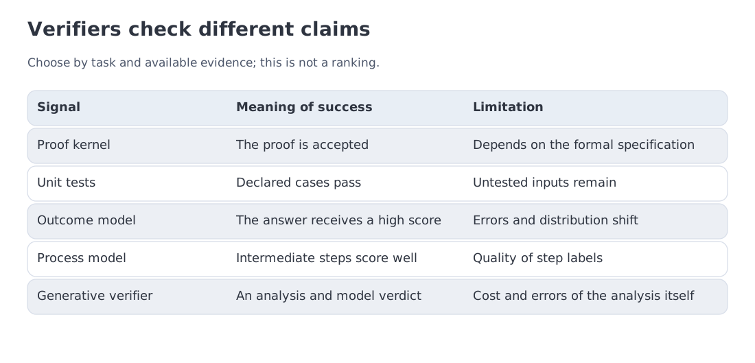 Verifier contracts: executable rules, outcome and process models, generative judges, and reasoning reward models.
Reasoning RL is most straightforward when rewards are objectively checkable. Creative writing, advice, and aesthetics do not have a unique ground truth; there, a learned verifier represents a preference or rubric rather than mathematical correctness.
16. Distilling reasoning traces
DeepSeek released six dense R1-Distill models ranging from 1.5B to 70B, trained using data generated by R1. The release made a practical route visible: successful long-form solutions from a strong teacher can become supervised data for a smaller student. DeepSeek-R1, 2025
A student can absorb:
- the surface format of decomposition;
- recurring intermediate operations;
- habits of checking and revision;
- length and style distributions;
- domain heuristics represented in the traces.
Distillation updates the student's weights. Its data can teach new knowledge, representations, and procedures, so the starting checkpoint is not an immutable capability ceiling. What the student does not receive is the teacher's parameters or a guarantee of equivalent behavior. Capacity, data quality and diversity, the training objective, and the evaluation distribution all affect the result.
This differs from §8: extending inference with fixed weights changes work on one request, whereas distillation changes the function used for future requests. Both benefit from verified solutions, but they spend computation at different stages.
It helps to separate three claims:
- format transfer: the model produces an organized reasoning trace;
- procedure transfer: it applies patterns present in the training data;
- out-of-distribution generalization: this must be tested on new task families and depends on model capacity, data diversity, and the training objective.
A “reasoning distillate” should therefore be evaluated as its own model, including quality, token efficiency, calibration, and failure modes.
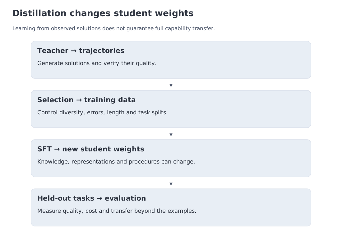 Teacher traces transfer useful procedures, with weight updates and separate evaluation of the resulting student.
17. Reading a model's reasoning passport
As of 11 October 2026, “supports reasoning” is not enough information for deployment. A useful passport answers at least seven questions.
- How is reasoning enabled? Is it always on, adaptive, selected by effort level, or controlled by a token target? Can it be disabled?
- What kind of compute scales? One longer trajectory, several candidates, subagents, or a combination?
- What is exposed? Full traces, summaries, a separate field, opaque signatures, or only the final answer?
- What is billed and limited? Do reasoning tokens count as output and consume
max_tokens? Are they reported in usage metadata? - How does it interact with tools? Must the client preserve complete assistant messages, signatures, or reasoning items across calls?
- What are the systems consequences? Measure median and tail latency, reasoning length, KV footprint, and concurrency on the actual workload.
- How was quality compared? Equal cost, equal wall-clock time, equal generated tokens, or unrestricted settings? Were tools and multiple agents allowed?
This passport separates model capability from serving policy. It also prevents accidental comparisons between single-trajectory depth and multi-agent breadth.
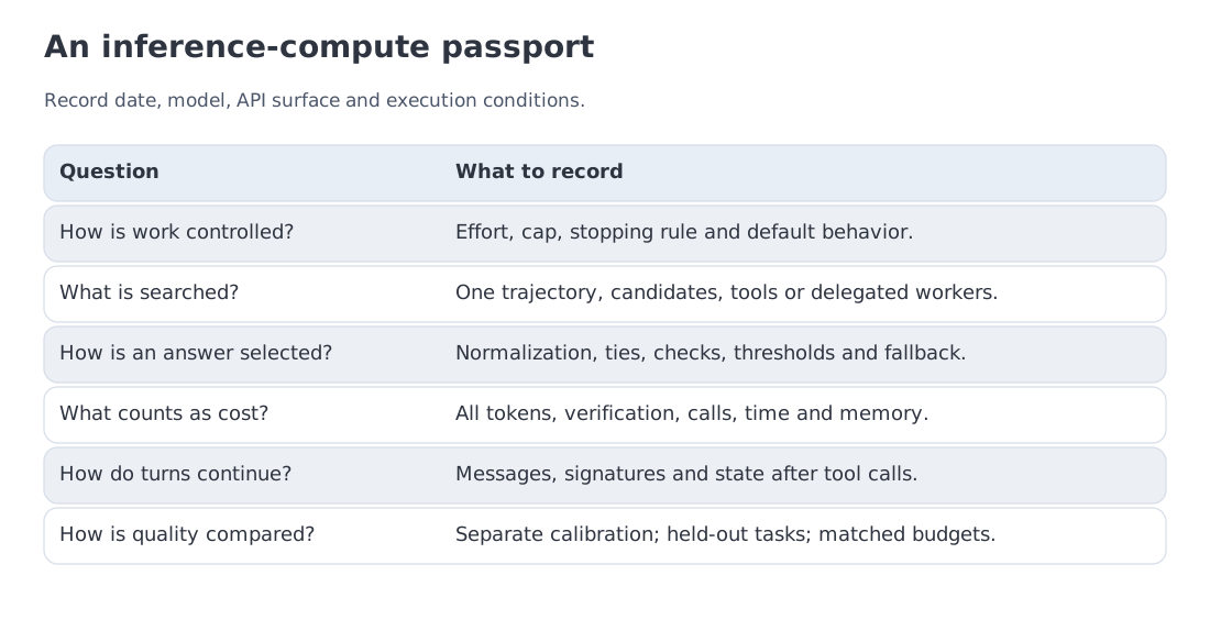 Each row records part of a reproducible protocol; a model name does not replace these details.
20. Key takeaways and sources
- Test-time compute is a real scaling axis, but not a free substitute for a capable base model.
- Sequential depth, parallel breadth, and adaptive allocation address different failure modes.
- Repeated sampling raises coverage; selection quality determines how much of that coverage becomes accuracy.
- Tie handling, answer normalization, and sample dependence are part of the self-consistency algorithm.
- A verifier can become the bottleneck—and can itself be exploited.
- With fixed decode rate and full-history caching, decode time and KV memory grow linearly with generated length, while the product impact on latency and concurrency can be severe.
- Adaptive budgets are valuable because workload difficulty is heterogeneous and quality need not be monotonic in chain length.
- Distillation transfers visible procedures and traces, not the teacher's full capability.
- Comparing reasoning systems requires a passport covering controls, depth versus breadth, visibility, billing, tool continuity, systems cost, and evaluation protocol.
Primary sources:
- OpenAI — Learning to reason with LLMs
- DeepSeek-R1
- Scaling LLM Test-Time Compute Optimally
- Large Language Monkeys
- s1: Simple Test-Time Scaling
- Let's Verify Step by Step
- Generative Verifiers
- RM-R1: Reward Modeling as Reasoning
- OpenAI API model guidance
- Anthropic thinking documentation
- Gemini API thinking documentation
- Kimi K3 quickstart
- Thinking Machines — Inkling
- Meta — Muse Spark 1.1
Snapshot for current API details: 11 October 2026.
Landscape verified: October 11, 2026. Current API controls were checked against official documentation and research results against primary publications. Teaching estimates for latency, memory, and cost are reproduced by local calculations and apply only under the stated assumptions.