Module 10. KV Caches and Efficient Inference
“Modern LLMs” course · Module 10 lecture · edition 2026.10.25
What this module is about. Module 9 ended when the training run produced a model. That is only the beginning of the system problem. A deployed model must now answer many requests at once, preserve latency targets, reuse work when possible, and fit both its weights and a growing amount of per-request state into a finite memory hierarchy.
The key object is the KV cache. It removes the need to recompute the entire prefix at every autoregressive step, yet it also grows with context length and concurrency. We will derive its size from the attention geometry, place it inside a simple bandwidth model, locate the point at which batching stops amortizing the weights efficiently, and then follow the engineering consequences: paged allocation, prefix reuse, tiered storage, prefill/decode disaggregation, quantization, and eviction.
Every number in the worked examples belongs to an explicit teaching scenario. A bandwidth ceiling is not a benchmark, a vendor result is not an independent measurement, and an API price is not a permanent property of the underlying mechanism. Keeping those categories separate is part of the lesson.
Useful background. Module 5 supplies the attention layouts, Module 8 explains recurrent state, and Module 9 introduces lifecycle inference cost. We develop roofline reasoning here: both arithmetic and data movement limit runtime. With ideal overlap, the larger of the two times gives a lower bound.
Reading routes
First pass — follow a token into the serving system. Read §§1, 3–9, §11 up to “Implementation examples”, and the main takeaways in §20. Return to the “Compression” and “Storage tiers” paragraphs and the storage-tier parts of the figure after §§10 and 14–15. Follow the chain from retained state to bytes, bandwidth, allocation, and reuse. In §6, start with the throughput equation and table; leave the FLOP refinement for a return visit. Work through E1 and check E2 in the notebook.
Second pass — implement and challenge the assumptions. Add the historical context (§2), refined arithmetic (§§6, 9), storage hierarchy (§10), code (§§12–13), and compression (§§14–15). Run every notebook cell, including invalid shapes, page exhaustion, and rollback beyond the retained window. Then solve E3 and run both project demos.
Reference use. Consult §§16–17 when recording an engine/model configuration, §18 to test your understanding, and §19 for projects. API terms and connector support have a verification date; each calculation has explicit assumptions.
1. Motivation: a generated token is a memory transaction
During training, thousands of tokens can contribute to large matrix multiplications before the weights must be fetched again. Autoregressive decoding has a less favorable shape. Each active sequence asks for one new token. In a dense model with full attention, that step reads nearly all weights and the accumulated keys and values of the available context. MoE and bounded-memory mechanisms read different subsets, so architecture must remain explicit in the estimates. The amount of arithmetic per byte can become very small even on an accelerator with enormous peak FLOP/s.
This is why parameter count alone is a poor predictor of serving behavior. Two models with similar active parameters may store radically different amounts of history. A conventional multi-head attention model keeps one key and one value vector for every head at every layer. GQA reduces the number of KV heads. MLA stores a compressed latent representation. Hybrid architectures may combine full-attention layers with recurrent or convolutional state. Before estimating latency or capacity, we must first ask a seemingly mundane question: what exactly is retained after each token?
We call prompt processing prefill and one-token-at-a-time generation decode. HBM is the accelerator's high-bandwidth memory; DRAM is CPU main memory. A service-level objective (SLO) sets a target such as an upper latency percentile. Section 5 connects these terms to user-visible timing.
The answer affects three quantities at once.
First, it affects capacity. A cache that is modest at 8K tokens may exceed the weight payload at one million tokens. Second, it affects bandwidth. Decoding must read the relevant state repeatedly, so longer contexts lower the memory-bound throughput ceiling. Third, it affects scheduling. A server that mixes long prompts, short prompts, cache hits, and growing outputs needs a memory manager rather than a single preallocated tensor.
The rest of the module follows that chain. We begin with bytes per token, turn those bytes into a speed ceiling, and then ask what a serving stack can do about the result.
2. The historical arc: four successive bottlenecks
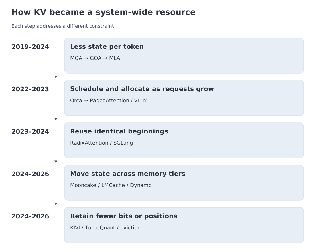 The inference line: MQA reduces KV heads; GQA becomes a practical compromise; Orca introduces iteration-level scheduling; PagedAttention brings block allocation and sharing; MLA compresses stored attention state; Mooncake, LMCache, and later disaggregated runtimes turn KV into a distributed data object.
The first wave changed the architecture. Multi-Query Attention (MQA) showed that all query heads could share a much smaller set of key/value heads. Grouped-Query Attention (GQA) retained several KV groups and offered a better quality–memory compromise for many dense models. Multi-head Latent Attention (MLA) went further by storing a latent representation from which the required key/value information can be reconstructed.
The second wave changed the scheduler. Orca observed that sequences in a batch do not finish together and that waiting for a whole batch to complete wastes capacity. Its iteration-level scheduling allowed the active set to change after every decode step. The modern term continuous batching describes this family of schedulers: completed requests leave, new requests enter, and the GPU keeps doing useful work.
The third wave changed the allocator. Variable-length sequences make contiguous KV buffers expensive. PagedAttention borrowed the central idea of virtual memory: a logical sequence can be represented by a table of fixed-size physical blocks. This reduces fragmentation, supports copy-on-write sharing, and lets the scheduler grow sequences without reserving their maximum length in advance. vLLM made this design widely accessible; SGLang’s RadixAttention emphasized structured reuse of common prefixes.
The fourth wave changed the scope of the cache. Once the KV state became valuable enough, keeping it inside one process was no longer sufficient. LMCache added external storage and transfer paths. Mooncake treated CPU memory, local storage, and networked resources as a global KV pool. Prefill/decode disaggregation placed the two phases on different worker pools and turned KV transfer into an explicit systems operation. By 2026, context state had become a first-class distributed resource with its own placement, routing, and lifecycle policies.
No wave made the previous ones obsolete. A current serving system typically combines architectural reduction, iteration-level scheduling, paged allocation, prefix reuse, and a memory hierarchy. Each mechanism removes a different term from the cost.
3. A bridge to classical systems: pages, caches, and queues
Three older systems ideas provide a useful mental model.
Virtual memory. A process sees a contiguous address space even though physical pages may be scattered. PagedAttention applies the same separation to a sequence: logical token positions map to fixed-size KV blocks, and the blocks need not be adjacent. Sharing a prefix then means sharing page-table entries; copy-on-write creates a private block only when one branch diverges.
Cache hierarchies. HBM is fast and scarce, CPU DRAM is larger and slower, local SSD is larger again, and remote storage adds network cost. Moving KV between these levels is governed by the same questions that appear in databases and operating systems: expected reuse, transfer latency, eviction policy, and prefetch timing. The unusual feature is the object being cached: a representation whose recomputation cost grows with the prefix length.
Queueing and phase separation. Prefill and decode stress the accelerator differently. A long prefill can occupy compute resources for a relatively large contiguous interval, while interactive decode consists of many short latency-sensitive steps. A system may have excellent average throughput and still violate user-facing latency objectives because the two phases interfere in the tail. Goodput—the work completed while meeting the service-level objective—is therefore more informative than raw throughput alone.
These analogies are not just pedagogical decoration. They tell us which knobs to expect: block size, admission control, queue discipline, cache key, time-to-live, placement tier, prefetch, and backpressure.
4. Formalism and worked example A: how many bytes does one token add?
For ordinary MHA or GQA, let
- be the number of attention layers;
- the number of KV heads per layer;
- the head dimension;
- the number of bytes per stored scalar.
Each token contributes one key vector and one value vector at every attention layer, so
The factor of two is not an approximation: it is the pair and . What is architecture-dependent is the object represented by . MLA, recurrent attention variants, and hybrid models may store a latent or several kinds of state instead of ordinary key/value heads; those cases require their own geometry.
For bf16, . The teaching configurations give the following ladder:
| Architecture | Configuration | Stored state per token | Interpretation |
|---|---|---|---|
| 70B MHA equivalent | , , | 2,560 KiB | full KV for every attention head |
| Llama-3.3-70B GQA | , , | 320 KiB | eightfold reduction from the MHA equivalent |
| Llama-3-8B GQA | , , | 128 KiB | reference geometry for the roofline example |
| DeepSeek-V3 MLA | model-specific latent + RoPE state | 68.625 KiB | a separate MLA calculation, not the GQA formula |
For MLA, use : with 61 layers, a 512-dimensional latent, 64 positional coordinates, and 2 bytes per scalar, the result is B = 68.625 KiB/token. A recurrent layer instead retains a fixed state; it has no constant per-token KV slope. A hybrid needs both terms.
Throughout the examples, 8K = 8192, 32K = 32768, 128K = 131072, and 1M = 1,000,000 tokens. These length labels are separate from memory units. For equal-length requests, .
The units matter. Dividing bytes by gives KiB; accelerator and operating-system tools often report binary capacities even when product names use decimal “GB”.
Now consider the 70B GQA row. It stores 327,680 bytes per token. At batch one:
- 8,192 tokens require 2.5 GiB;
- 32,768 tokens require 10 GiB;
- 131,072 tokens require 40 GiB;
- 1,000,000 tokens require 327.68 GB, or about 305.18 GiB.
A bf16 weight payload of 70 billion parameters is roughly 140 GB. The cache crosses that weight payload at
Beyond that point, a single sequence carries more KV state than the model’s weights. Concurrency multiplies the cache again. This is the arithmetic behind the statement that long-context serving is a memory problem.
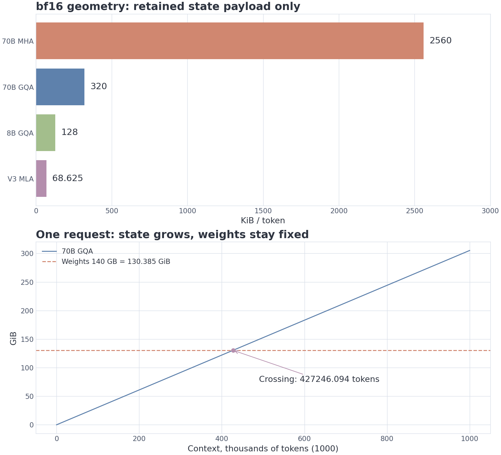 The top panel compares KiB per token across MHA, GQA, and MLA examples. The bottom panel shows the 70B GQA cache growing through the bf16 weight payload.
5. One request, two computational regimes
An inference request has two phases, and treating them as one homogeneous workload hides the central scheduling problem.
During prefill, the model processes the prompt and constructs its state. Many positions participate in matrix operations at once, so the accelerator can often use its compute units efficiently. The user experiences this phase through time to first token (TTFT).
During decode, the model adds one token per active sequence per step. The weights are read again, and attention reads the accumulated KV state. Arithmetic no longer grows in proportion to the amount of data moved, so the phase is often memory-bandwidth bound. The user experiences it through inter-token latency (ITL) or the corresponding stream rate after the first token.
The distinction is workload-dependent, not metaphysical. Very short prompts may not make prefill fully compute-bound; large batches and fused kernels can improve decode utilization; sparse or recurrent architectures alter the state traffic. Nevertheless, the two-regime model is a useful first approximation because it explains why one long prompt can disturb many otherwise smooth decode streams.
A service-level objective may constrain TTFT, ITL, a percentile of end-to-end latency, or all three. Interactive chat, offline batch generation, and agent rollout generation place different weights on these metrics. The scheduler should therefore maximize useful work under the chosen constraints, not merely display the largest aggregate token count.
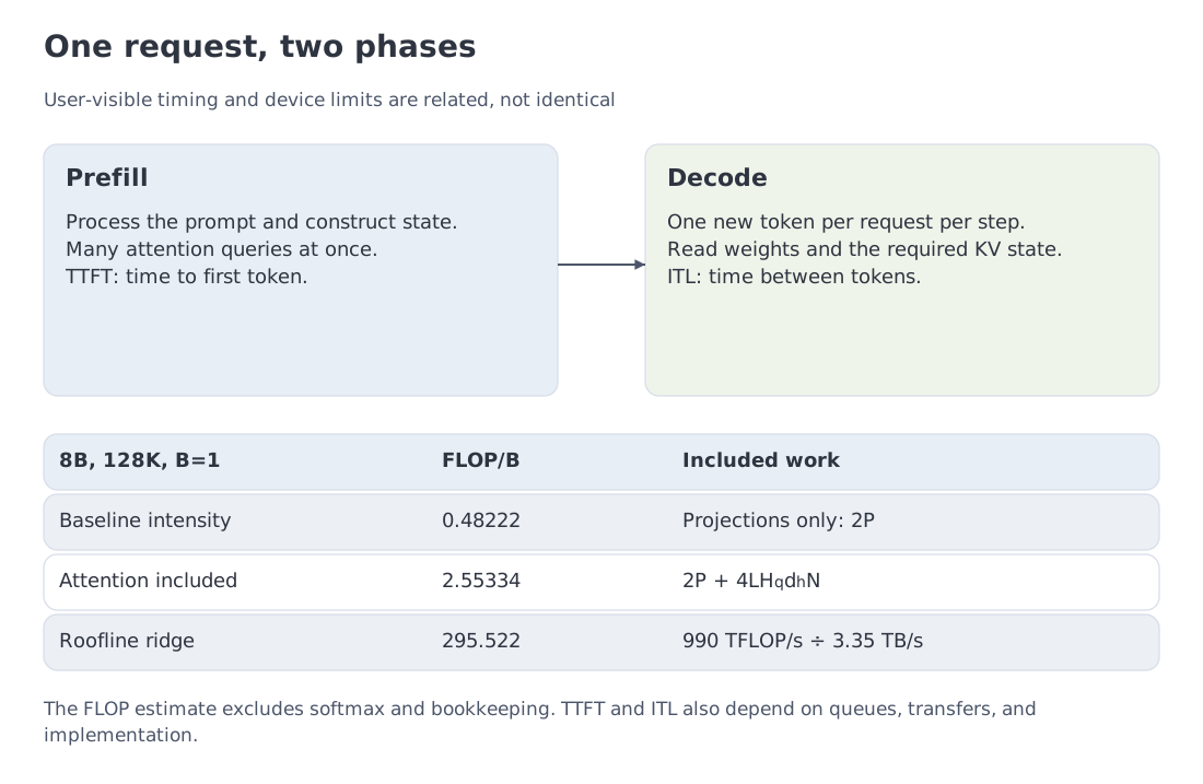 Prefill builds the prompt state with high matrix reuse; decode advances one token at a time and repeatedly reads weights plus KV. TTFT and ITL expose the two phases to the user.
6. Worked example B: the bandwidth ceiling and the KV term
Take an 8B bf16 model with a 16 GB weight payload, the 128 KiB/token geometry above, and an H100-like memory bandwidth of 3.35 TB/s. We deliberately use a simple model: one decode step reads the weights once and reads the resident KV state once. Ignoring compute and all other traffic gives the aggregate bandwidth ceiling
where is the number of active sequences, the context length, the weight bytes, and the memory bandwidth. For batch one this reduces to
The resulting ceilings are:
| Context | Cache traffic per sequence | Ceiling at batch 1 |
|---|---|---|
| 0 | 0 | 209.4 tok/s |
| 8K | 1.0 GiB | 196.2 tok/s |
| 128K | 16 GiB | 101.0 tok/s |
| 1M | 122.1 GiB | 22.8 tok/s |
These are not expected wall-clock measurements. They omit kernels, synchronization, activation traffic, scheduler overhead, and the fact that not every implementation reads every byte in exactly this way. Their value is diagnostic: the equation shows why the ceiling falls as context grows even though the weights have not changed.
The 0-context row is a weights-only baseline, not a usable prompt. The 1M row requires 136.97 GiB for weights plus KV before reserve and cannot run on the 80-GiB device assumed by the capacity example.
Refinement: context also adds attention FLOPs
Here counts parameters and counts query heads. The estimate covers projections; the second term counts QK and AV, with two FLOPs per multiply-add. counts keys visible to the current query, including its own position; the model does not distinguish the new KV write from subsequent reads. Softmax, normalization, and bookkeeping remain excluded.
Arithmetic intensity measures operations per byte read. Assume a peak of 990 TFLOP/s and bandwidth of 3.35 TB/s. Their ratio is the roofline ridge: the intensity where ideal compute and memory times coincide. Below it, memory takes longer.
For the 8B example at , , , , and give about 84.7195 GFLOP per step and 2.55334 FLOP/B. The roofline ridge is FLOP/B, about 115.74 times higher. Keeping only gives 0.48222 FLOP/B and a 612.84 ratio: useful as a projection-only baseline, but incomplete as a decode intensity. GQA reduces KV heads for storage; attention arithmetic here uses query heads.
With ideal overlap, a step takes at least . Actual kernels add work and traffic. The model identifies a scale and a bottleneck; it does not promise latency.
7. Batch economics: where weight amortization stops being the whole story
Batching helps because several sequences can share one read of the weights. If KV traffic were zero, aggregate throughput would initially grow almost linearly with batch size. The denominator above shows why the gain eventually bends: each additional sequence brings its own context state.
Set total KV traffic equal to the weight payload:
This is not a hard optimum. It marks a useful transition: before , reading the weights dominates the denominator; after it, per-request KV traffic increasingly controls the gain.
For the teaching scenario:
- at 8K, ;
- at 32K, ;
- at 128K, .
The last value is the striking one. At 128K, one sequence already brings roughly as much KV traffic as the weights. Batching remains useful, but it no longer behaves like free weight amortization.
At batch 32 and 8K, the model predicts 2,128.7 tok/s rather than the 6,700 tok/s one would obtain by multiplying the zero-KV batch-one ceiling by 32. The ratio, about 3.15×, is the “KV tax” in this particular arithmetic scenario.
is aggregate throughput. With equal service, each request receives : batch 32 therefore gives 66.52 tok/s per request, corresponding to an ideal 15.03 ms step. Check capacity separately: the hypothetical 80-GiB device, less 16 GB of weights and an 8-GiB reserve, holds at most 57, 14, and 3 requests at 8K, 32K, and 128K; it holds none at 1M. The 80-GiB capacity is an explicit teaching input, not a relabeling of every H100 specification.
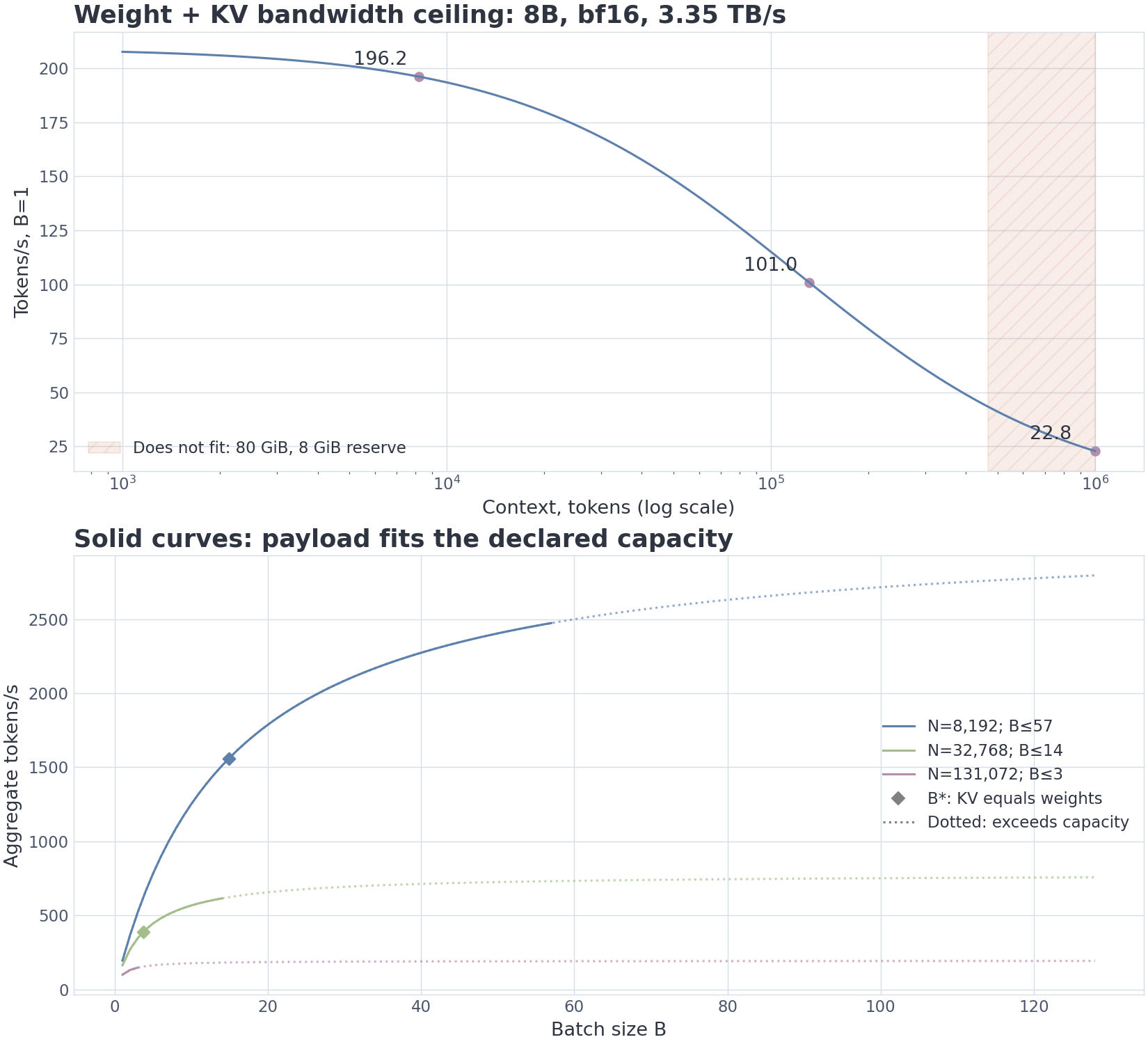 Top: the bandwidth ceiling falls as context grows. Bottom: aggregate throughput rises with batch, but the curve bends earlier for longer contexts. Diamonds mark equal KV and weight traffic; dotted segments exceed the stated memory capacity.
8. PagedAttention: decouple logical length from physical placement
A naïve server can reserve one contiguous KV buffer per request, sized for that request’s maximum allowed context. The policy is simple and usually wasteful. Most requests finish before the limit, sequences grow at different rates, and free regions become fragmented. Worse, a request that needs one more token may be unable to extend even when enough memory exists elsewhere.
PagedAttention replaces the contiguous buffer with a table of fixed-size blocks. The logical token positions remain ordered, but their physical blocks may sit anywhere in the pool. A request receives blocks as it grows, not when it is admitted.
The internal waste is then bounded by the unused tail of the final block. With block size , a sequence wastes at most token slots. For a 32K maximum context, a request that currently contains 2K tokens would waste
under full contiguous reservation. That exact 2048-token sequence fills 16-token pages without waste. Now consider a different workload: lengths average 2048, with uniform residues modulo 16. The mean unused tail is 7.5 slots, so the ratio of expected unused to expected allocated slots is approximately
Each figure belongs to its own assumptions. They are not universal measurements of vLLM. The original PagedAttention work reported near-zero memory waste and 2–4× throughput improvements over its comparison systems, but the realized gain depends on length distribution, block size, scheduler, and hardware.
Keep the workloads distinct. A sequence of exactly 2048 tokens fills 16-token blocks with zero waste. The 0.365% result assumes varying lengths with mean 2048 and uniform remainders, leaving 7.5 slots unused on average. It divides expected unused slots by expected allocated slots, rather than averaging each request's waste fraction. Dividing by 2048 instead measures overhead relative to useful payload (0.366%).
Block allocation also enables copy-on-write. Two branches can point to the same complete prefix blocks. A physical copy is needed only when a branch must modify a shared partial block. This matters for beam-like branching, speculative decoding, and any workflow that forks a common conversation state.
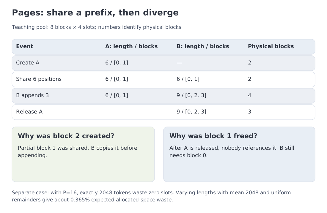 Logical sequences map through page tables into a shared block pool. The example contrasts maximum-length reservation with demand allocation and shows prefix sharing through copy-on-write.
9. Prefix caching: do not rebuild an identical beginning
Many requests begin with the same material: a system instruction, a few-shot demonstration set, a tool schema, a large document, or an earlier part of a conversation. If the token sequence and every computation-relevant setting match, the corresponding KV state can be built once and reused.
Consider 8192 input tokens, with 7680 already cached and 512 left to process. The projection-only estimate gives 132.396 ms versus 8.275 ms, a ratio of 16. Reusing a prefix does not remove the suffix queries' attention to that prefix. With suffix length and cached length , causal attention costs:
There are allowed query–key pairs. The bracket is twice that count. Each pair costs FLOPs for QK and AV, leaving the factor when applied to the bracket. Softmax and overhead are still excluded. For 32 layers, 32 query heads, dimension 128, and 990 TFLOP/s, full prefill gives 150.168 ms and the cached suffix gives 10.427 ms: a 14.402 ratio. These remain arithmetic estimates. KV transfer, lookup, queues, and achieved FLOP/s determine observed TTFT.
Public APIs now expose caching rules for matching, retention, writes, and reads. Section 16 gives the OpenAI example. Kimi K3 also prices cache hits separately; Moonshot reports over 90% hits on its coding workloads. That is a service-specific observation, not a forecast for another application's traffic.
Exact-prefix matching leads to a practical prompt-layout rule: place stable instructions and reusable documents first, and put request-specific material later. The rule has limits. A provider or engine may hash blocks differently, include model settings in the cache key, impose a minimum length or time-to-live (TTL), restrict sharing scope, or invalidate entries when images, tools, or model versions change. The relevant documentation must therefore be read as part of the serving contract.
A block is contextual: identical token IDs after different earlier tokens need not produce the same K/V. A cache key must distinguish the model and adapters, positional configuration, and preceding prefix; sharing scope is a separate contract.
Prefix caching offers little when the common portion is small, tokenization differs, or every request carries unique context. A process-local cache is also bounded by the process’s memory and lifetime. The next step is to make the state portable beyond one engine instance.
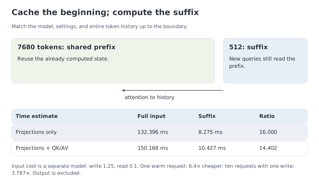 Stable prompt components form a reusable prefix; changing material remains at the end. The diagram shows the 8K-to-512 arithmetic reduction and the exact-match constraint.
10. Tiered placement: when HBM is only the first level
If useful KV state does not fit in HBM, the system can recompute it later or preserve it on a cheaper tier. The second option creates a hierarchy such as
Capacity rises along the hierarchy, while access latency and transfer cost rise as well. Offloading is therefore not automatically beneficial. Keeping a block is worthwhile when its expected reuse value and recomputation cost exceed the cost of writing, storing, and restoring it.
LMCache separates KV storage and transfer from a particular inference engine. A deployment may use CPU memory or disk on the same node, a separate LMCache server shared by several vLLM instances, or external backends such as Redis/Valkey, Mooncake, S3-compatible storage, NIXL, or GDS. Some configurations reuse exact prefixes; CacheBlend extends the idea to selected blocks that reappear in different positions with partial recomputation. The important abstraction is that KV becomes managed data rather than a private tensor owned by one attention kernel.
Mooncake applies the idea at distributed-platform scale. In the published Kimi system, prefill and decode are separated, idle CPU memory and storage resources form a global KV pool, and a transfer engine moves state across the network. The scheduler considers service-level objectives and can reject requests early when the available capacity cannot meet them. In the FAST 2025 paper, the authors report 59–498% higher effective serving capacity in their trace-driven experiments while meeting the selected SLOs, operation across thousands of nodes, and more than 100 billion tokens served per day. These are results for the authors’ system and workloads, not generic factors for any cluster.
NVIDIA’s CMX announcement of 16 March 2026 describes a hardware-and-network context-memory layer built around BlueField-4 and Spectrum-X for the Vera Rubin ecosystem. NVIDIA reports up to 5× higher tokens per second and energy efficiency against a chosen conventional storage design. At the time of the course snapshot, that figure is a vendor projection for a specific forthcoming platform rather than a broadly reproduced H100 result.
The systems principle is stable even when products change: a large context state needs an explicit placement policy, a transfer path, and a decision about whether retrieval or recomputation is cheaper.
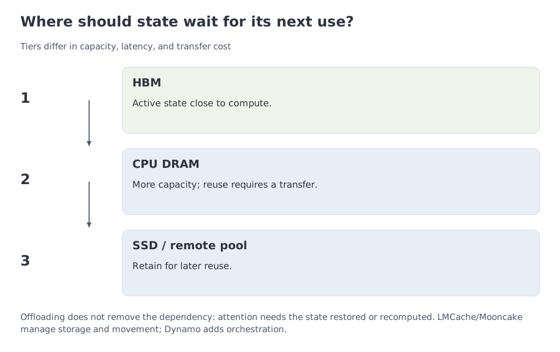 KV moves through HBM, CPU memory, local storage, and remote storage. LMCache and Mooncake provide software layers; CMX represents a hardware-oriented extension of the same hierarchy.
11. Prefill/decode disaggregation: give each phase its own pool
Return to the phases from §5. A long prefill in a shared queue can delay active decode streams. To isolate scheduling, start with two deliberately limited estimates: projection-only prefill at 132.396 ms and weight-read-only decode at 4.776 ms. Their serial sum, 137.172 ms, bounds the selected work; it is not a predicted interruption.
Chunked prefill lets the scheduler insert decode steps between prompt segments. Projections for 512 tokens give 8.275 ms, so the two selected estimates sum to 13.051 ms. Equal-size chunks are not equal-cost once attention is counted: later chunks see more history. The notebook checks that all 16 chunks sum to the full prefill's work; the final chunk's attention-inclusive estimate is 10.427 ms.
The prefill work has not vanished; it has been divided and interleaved so that its tail-latency effect is smaller.
A more structural remedy is prefill/decode disaggregation. Prefill workers can be configured for large prompt matrix operations and throughput; decode workers can be configured for low ITL and memory bandwidth. The KV state is transferred between the pools after prefill. Each pool can use a different tensor-parallel degree, admission policy, and batching strategy.
The separation is not free. KV transfer joins the critical path, the scheduler must know where each block resides, and network backpressure becomes part of request admission. For small loads or short prompts, one pool with continuous batching and chunked prefill may be simpler and faster.
Implementation examples
As of 11 October 2026, vLLM’s stable documentation still labels disaggregated prefill experimental, while exposing several KV connectors and independent TTFT/ITL tuning. NVIDIA Dynamo 1.0, released on 16 March 2026, orchestrates vLLM, SGLang, and TensorRT-LLM, uses NIXL for data movement, and routes requests with KV locality in mind. NVIDIA reports up to 7× more requests served on Blackwell in a specific SemiAnalysis InferenceX DeepSeek-R1 configuration. That number belongs to the stated stack and protocol; it is not a universal multiplier for phase separation itself.
Connection to RL infrastructure. This module focuses on interactive and service inference. Large-scale rollout generation, actor/learner separation, policy staleness, and asynchronous queues are developed in RL for LLM, Module 12. The same memory and scheduling primitives reappear there under a different workload profile.
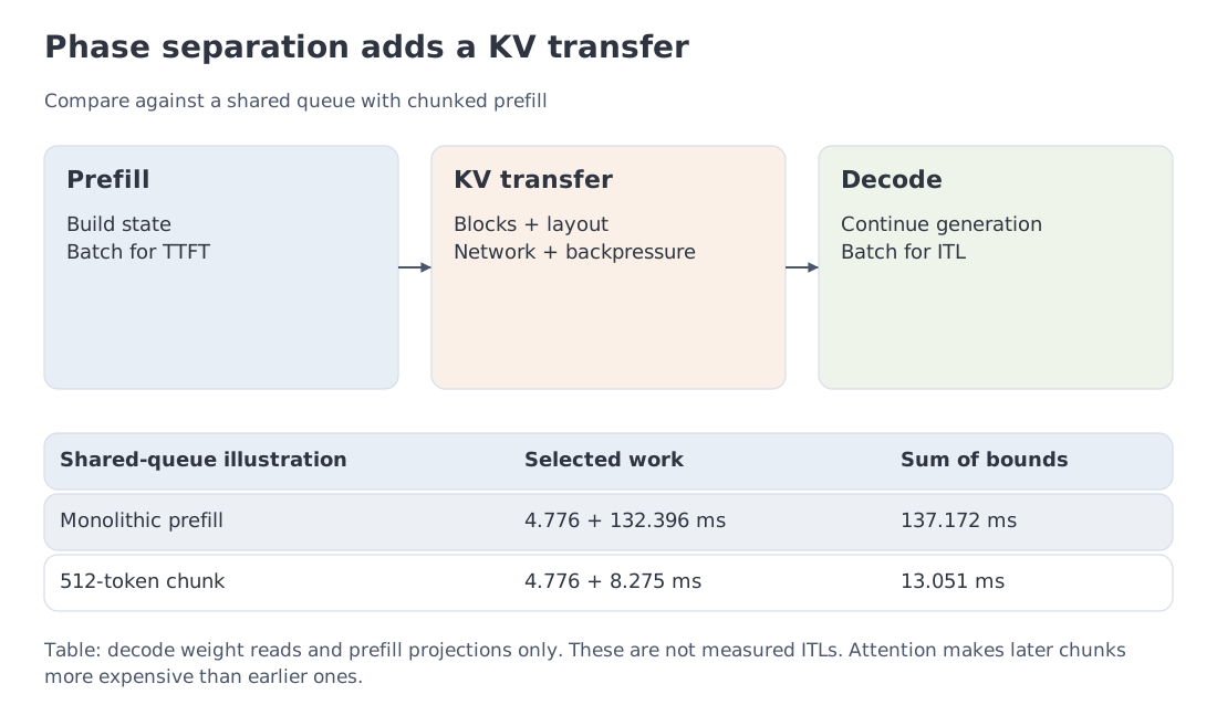 The prefill pool builds state, the transfer layer moves KV, and the decode pool advances streams. The lower panel compares monolithic and chunked interference in the teaching scenario.
12. Code (level 1): geometry, bandwidth, and private pages
Start with three small objects. KVGeometry counts bytes; decode_bandwidth_ceiling returns aggregate tokens per second; PagedKV allocates private pages as a sequence grows. It does not share prefixes. The notebook's PagedKVPool adds reference counts, copy-on-write, and allocation-failure atomicity.
"""Lecture-level geometry, bandwidth bound, and private page allocation."""
from dataclasses import dataclass, field
import math

def count(value, minimum=0):
    if isinstance(value, bool) or not isinstance(value, int) or value < minimum:
        raise ValueError(f"expected an integer >= {minimum}")
    return value

@dataclass(frozen=True)
class KVGeometry:
    attention_layers: int
    kv_heads: int
    head_dim: int
    bytes_per_element: int = 2

    def __post_init__(self):
        for value in (self.attention_layers, self.kv_heads, self.head_dim, self.bytes_per_element):
            count(value, 1)

    @property
    def bytes_per_token(self):
        return 2 * self.attention_layers * self.kv_heads * self.head_dim * self.bytes_per_element

def decode_bandwidth_ceiling(context_tokens, weight_bytes, geometry, bandwidth_Bps,
                             batch_size=1, kv_scale=1.0):
    """Aggregate tok/s, assuming one weight read and one KV read per step."""
    count(context_tokens); count(weight_bytes, 1); count(batch_size, 1)
    for value in (bandwidth_Bps, kv_scale):
        if isinstance(value, bool) or not math.isfinite(value) or value <= 0:
            raise ValueError("bandwidth and scale must be positive and finite")
    kv = geometry.bytes_per_token * context_tokens * batch_size * kv_scale
    if not math.isclose(kv, round(kv), rel_tol=0, abs_tol=1e-9):
        raise ValueError("the scaled payload must contain an integer number of bytes")
    return batch_size * bandwidth_Bps / (weight_bytes + round(kv))

@dataclass
class PagedKV:
    """Private logical pages only; the notebook adds sharing and copy-on-write."""
    n_blocks: int
    block_size: int = 16
    free: list = field(init=False)
    tables: dict = field(default_factory=dict, init=False)
    lengths: dict = field(default_factory=dict, init=False)

    def __post_init__(self):
        count(self.n_blocks, 1); count(self.block_size, 1)
        self.free = list(range(self.n_blocks - 1, -1, -1))

    def append_to(self, seq_id, total_tokens):
        count(total_tokens)
        hash(seq_id)
        if total_tokens < self.lengths.get(seq_id, 0):
            raise ValueError("append_to cannot shorten a sequence")
        table = self.tables.get(seq_id, [])
        needed = (total_tokens + self.block_size - 1) // self.block_size - len(table)
        if needed > len(self.free):
            raise MemoryError("not enough free blocks")
        self.tables.setdefault(seq_id, table)
        table.extend(self.free.pop() for _ in range(needed))
        self.lengths[seq_id] = total_tokens

    def release(self, seq_id):
        self.free.extend(self.tables.pop(seq_id))
        del self.lengths[seq_id]
Check that 2048 tokens fill exactly 128 pages of size 16, and that an allocation failure leaves all tables unchanged. The same minimal source is embedded and executed in the notebook.
The next bridge stores actual K/V tensors in a bounded window. Its attention check uses one query at a time; chunked multi-query attention needs its own mask and access to earlier positions. Rollback is valid only inside the retained interval and cannot recover an evicted prefix. Window movement never resets absolute positions.
NumPy → PyTorch · B17 — Bounded KV cache: append, window, and rollback
The cache stores K/V together with an absolute position range. A bounded window physically evicts the old prefix, while rollback truncates only the retained suffix.
import numpy as np
import torch
import torch.nn.functional as F
1. Explicit NumPy implementation
class NumpyKVCacheExplicit:

    def __init__(self, *, window: int | None = None) -> None:
        if window is not None and (isinstance(window, bool) or not isinstance(window, int) or window <= 0):
            raise ValueError("window must be a positive integer or None")
        self.window = window
        self.k = self.v = None
        self.start_pos = self.next_pos = 0

    def append(self, k_new, v_new):
        k_new, v_new = np.asarray(k_new), np.asarray(v_new)
        if k_new.ndim != 4 or k_new.shape != v_new.shape or min(k_new.shape) <= 0:
            raise ValueError("K and V need the same non-empty [B,H,T,D] shape")
        if k_new.dtype != v_new.dtype or not np.issubdtype(k_new.dtype, np.floating):
            raise ValueError("K and V need the same floating dtype")
        if self.k is not None:
            if self.k.shape[:2] + self.k.shape[3:] != k_new.shape[:2] + k_new.shape[3:]:
                raise ValueError("cache geometry changed")
            if self.k.dtype != k_new.dtype:
                raise ValueError("cache dtype changed")
        # Validate first; keep old state intact if an input is rejected.
        k = k_new.copy() if self.k is None else np.concatenate([self.k, k_new], axis=-2)
        v = v_new.copy() if self.v is None else np.concatenate([self.v, v_new], axis=-2)
        drop = max(0, k.shape[-2] - self.window) if self.window is not None else 0
        # A slice alone retains its backing allocation. Make owned bounded copies.
        self.k = k[..., drop:, :].copy() if drop else k
        self.v = v[..., drop:, :].copy() if drop else v
        self.start_pos += drop
        self.next_pos += k_new.shape[-2]
        return self.k, self.v

    def truncate(self, absolute_end: int) -> None:
        if isinstance(absolute_end, bool) or not isinstance(absolute_end, int):
            raise ValueError("absolute_end must be an integer")
        if not self.start_pos <= absolute_end <= self.next_pos:
            raise ValueError("rollback lies outside the retained interval")
        keep = absolute_end - self.start_pos
        if self.k is not None:
            self.k = self.k[..., :keep, :].copy()
            self.v = self.v[..., :keep, :].copy()
        self.next_pos = absolute_end

    @property
    def positions(self):
        return np.arange(self.start_pos, self.next_pos, dtype=np.int64)
The minimal cache exposes three pieces of state: retained K/V, the absolute position of the first retained token, and the next append position. After eviction, an owned copy releases this container's reference to the old backing buffer; slicing alone would retain it.
2. The same mathematics as explicit PyTorch operations
class TorchKVCacheExplicit:

    def __init__(self, *, window: int | None = None) -> None:
        if window is not None and (isinstance(window, bool) or not isinstance(window, int) or window <= 0):
            raise ValueError("window must be a positive integer or None")
        self.window = window
        self.k = self.v = None
        self.start_pos = self.next_pos = 0

    def append(self, k_new, v_new):
        if not isinstance(k_new, torch.Tensor) or not isinstance(v_new, torch.Tensor):
            raise TypeError("K and V must be tensors")
        if k_new.ndim != 4 or k_new.shape != v_new.shape or min(k_new.shape) <= 0:
            raise ValueError("K and V need the same non-empty [B,H,T,D] shape")
        if k_new.dtype != v_new.dtype or k_new.device != v_new.device or not k_new.is_floating_point():
            raise ValueError("K and V need the same floating dtype and device")
        if k_new.requires_grad or v_new.requires_grad:
            raise ValueError("this cache is for inference; detach inputs first")
        if self.k is not None:
            if self.k.shape[:2] + self.k.shape[3:] != k_new.shape[:2] + k_new.shape[3:]:
                raise ValueError("cache geometry changed")
            if self.k.dtype != k_new.dtype or self.k.device != k_new.device:
                raise ValueError("cache dtype or device changed")
        # Validate first; keep old state intact if an input is rejected.
        k = k_new.clone() if self.k is None else torch.cat([self.k, k_new], dim=-2)
        v = v_new.clone() if self.v is None else torch.cat([self.v, v_new], dim=-2)
        drop = max(0, k.shape[-2] - self.window) if self.window is not None else 0
        # A slice alone retains its backing allocation. Make owned bounded copies.
        self.k = k[..., drop:, :].clone() if drop else k
        self.v = v[..., drop:, :].clone() if drop else v
        self.start_pos += drop
        self.next_pos += k_new.shape[-2]
        return self.k, self.v

    def truncate(self, absolute_end: int) -> None:
        if isinstance(absolute_end, bool) or not isinstance(absolute_end, int):
            raise ValueError("absolute_end must be an integer")
        if not self.start_pos <= absolute_end <= self.next_pos:
            raise ValueError("rollback lies outside the retained interval")
        keep = absolute_end - self.start_pos
        if self.k is not None:
            self.k = self.k[..., :keep, :].clone()
            self.v = self.v[..., :keep, :].clone()
        self.next_pos = absolute_end

    @property
    def positions(self):
        device = self.k.device if self.k is not None else None
        return torch.arange(self.start_pos, self.next_pos, dtype=torch.long, device=device)
The tensor version validates dtype and device, then owns the retained window. This inference-only container rejects gradient-tracked inputs. A serving engine normally uses pages or preallocated buffers; the temporary concatenation here can exceed the final window's payload.
| Aspect | NumPy | PyTorch |
|---|---|---|
| Append | np.concatenate | torch.cat |
| Physical window | slice + owned copy | slice + clone |
| Absolute positions | Python integers | Python integers plus tensor state |
| Rollback | truncates the retained suffix | same contract |
| Storage allocation | reference container with copying | engines usually use a buffer or block pool |
Executable parity and edge-case check
np_cache = NumpyKVCacheExplicit(window=3); t_cache = TorchKVCacheExplicit(window=3)
for value in range(5):
    k_np = np.full((1,1,1,2), value, dtype=np.float64); v_np = k_np + 100
    np_cache.append(k_np, v_np); t_cache.append(torch.tensor(k_np), torch.tensor(v_np))
np.testing.assert_allclose(np_cache.k, t_cache.k.numpy())
np.testing.assert_array_equal(np_cache.positions, t_cache.positions.numpy())
assert (np_cache.start_pos, np_cache.next_pos) == (2,5)
np_cache.truncate(4); t_cache.truncate(4)
np.testing.assert_allclose(np_cache.k, t_cache.k.numpy())
rng = np.random.default_rng(17)
keys = rng.standard_normal((1,1,6,4)); values = rng.standard_normal((1,1,6,4)); queries = rng.standard_normal((1,1,6,4))
cache = TorchKVCacheExplicit(window=3)
for step in range(6):
    cache.append(torch.tensor(keys[..., step:step+1, :]), torch.tensor(values[..., step:step+1, :]))
    cached = F.scaled_dot_product_attention(torch.tensor(queries[..., step:step+1, :]), cache.k, cache.v)
    lo = max(0, step - 2)
    full = F.scaled_dot_product_attention(torch.tensor(queries[..., step:step+1, :]), torch.tensor(keys[..., lo:step+1, :]), torch.tensor(values[..., lo:step+1, :]))
    torch.testing.assert_close(cached, full)

# Rejected input must not mutate state; rollback cannot resurrect evicted tokens.
for cache_type, convert in ((NumpyKVCacheExplicit, np.asarray), (TorchKVCacheExplicit, torch.tensor)):
    c = cache_type(window=3)
    c.truncate(0)
    x = convert(np.ones((1,1,5,2), dtype=np.float64))
    c.append(x,x)
    assert (c.start_pos,c.next_pos) == (2,5)
    for bad in (-1,1,6,2.5,True):
        try: c.truncate(bad)
        except ValueError: pass
        else: raise AssertionError("invalid rollback accepted")
    assert (c.start_pos,c.next_pos) == (2,5)
    try: c.append(convert(np.zeros((1,2,1,2))),convert(np.zeros((1,2,1,2))))
    except ValueError: pass
    else: raise AssertionError("geometry change accepted")
    c.truncate(2)
    assert c.k.shape[-2] == 0
    c.append(convert(np.ones((1,1,1,2))),convert(np.ones((1,1,1,2))))
    assert (c.start_pos,c.next_pos) == (2,3)
    for window in (0,-1,2.5,True):
        try: cache_type(window=window)
        except ValueError: pass
        else: raise AssertionError("invalid window accepted")
a = NumpyKVCacheExplicit(window=3)
a.append(np.ones((1,1,10,2)),np.ones((1,1,10,2)))
assert a.k.flags.owndata and a.k.nbytes == 3*2*8
t = TorchKVCacheExplicit(window=3)
t.append(torch.ones(1,1,10,2),torch.ones(1,1,10,2))
assert t.k.untyped_storage().nbytes() == t.k.numel()*t.k.element_size()

print("B17 window, ownership, rollback, and invalid inputs: PASS")
Complete executable file: m10_cache_bridges.py
14. Compression I: eviction changes which history exists
When full state cannot be retained even with a memory hierarchy, the server may keep only a subset of positions. This is the strongest form of compression: once a KV entry is removed, recovering it requires recomputing the relevant prefix.
StreamingLLM keeps a small set of initial attention-sink tokens together with a sliding recent window. The rule is cheap and predictable. H2O keeps recent tokens plus heavy hitters with high accumulated attention mass. SnapKV estimates prompt-token importance from an observation window. Ada-KV and PyramidKV distribute a limited retained-cache budget across heads or layers.
Selecting pages to read is a different operation. QUEST retains all KV entries and uses the current query plus key summaries to choose pages for approximate attention. It reduces traffic on this step, not the stored history; a page skipped now may be useful to the next query. Selection overhead and approximation error must both be evaluated.
No policy is universally best. The notebook uses a deterministic 16-position example with a budget of eight. The simplified top-mass rule retains , while a positional “first four plus last four” rule keeps and loses heavy hitters . The example does not prove that H2O wins generally; it demonstrates the difference between content-aware and position-only decisions.
Results published in 2025–2026 add two cautions. Reasoning workloads can be especially sensitive to eviction, and compression may lengthen the generated reasoning chain even when final accuracy is preserved. Another line of work shows that protecting structural prompt boundaries can matter as much as the scoring rule. Evaluation must therefore include the real prompt format, long decode, and total generated-token cost—not only retrieval accuracy on a short benchmark.
The notebook's top-mass rule ranks a supplied score vector. It is not full H2O: it has no online score updates or separate recent-token quota. The project demo measures attention-output error, rather than retained K/V norm, and includes a query shift that makes historical importance misleading.
15. Compression II: quantization, low rank, and the order of operations
Eviction reduces the number of positions. Quantization keeps the positions but represents each one with fewer bits.
KIVI uses asymmetric 2-bit quantization: keys are quantized per channel and values per token. The paper reports up to 2.6× lower peak memory including weights, up to 4× larger batches, and 2.35–3.47× higher throughput on the evaluated workloads. The factors are smaller than the raw 16/2 ratio because the system still stores weights, scales, metadata, and a residual full-precision window and pays kernel overhead.
TurboQuant treats KV compression as streaming vector quantization. PolarQuant transforms vectors into a quantization-friendly representation, while QJL corrects dot-product estimates. The paper reports a near-lossless regime around 3.5 bits per channel and small degradation at 2.5 bits. Separately, Google Research reports up to 8× faster attention-logit computation with four-bit keys than with unquantized 32-bit keys on H100. That result concerns one operation, not the throughput of the whole model.
The notebook asks a simpler question: how would ideal three-bit storage change the bandwidth ceiling? Scaling the KV payload by takes 128 KiB per token to 24 KiB. At 128K context, the ceiling rises from about 101 to 174 tokens/s. This estimate excludes metadata and quantization-kernel overhead and makes no claim about output quality; actual memory use, speed, and quality must be measured together.
Low-rank methods attack another redundancy: the stored vectors may lie near a lower-dimensional subspace. They can be attractive when the projection cost and reconstruction kernels are well optimized, but rank is workload- and layer-dependent.
The practical order of levers is useful:
- architecture — reduce the state the model creates, through GQA, MLA, or another mechanism;
- quantization or low rank — preserve positions while reducing bytes per position;
- placement — move colder state to a slower tier;
- eviction — remove positions only when the previous levers are insufficient.
The order is not a theorem. It is a risk ordering: later steps are more likely to make specific long-range information unavailable.
Optional depth. Rate–distortion reasoning and the distinction between lossy coding and task-aware distortion are developed in Information Theory for ML, Modules 6–7. The present module uses only the engineering consequence: fewer bits buy capacity at the price of controlled representation error.
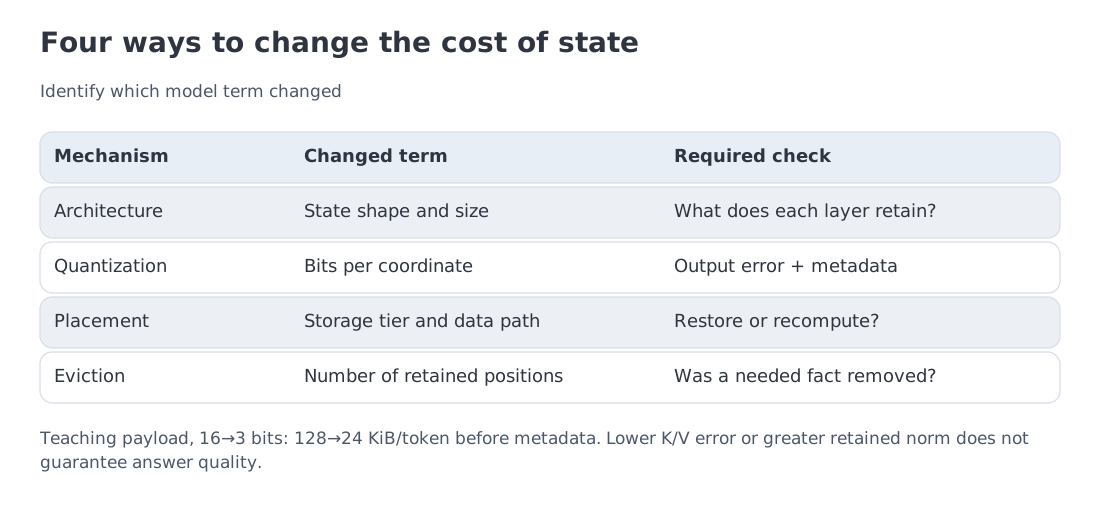 Four different levers act on four different quantities: architecture changes the state definition, quantization changes bytes per coordinate, placement changes location, and eviction changes the set of retained positions.
16. Engines and cache contracts: a dated map, not a permanent ranking
Serving software changes faster than the arithmetic. A useful map therefore describes responsibilities rather than declaring a single winner.
| Layer | Representative systems | Main responsibility |
|---|---|---|
| execution engine | vLLM, SGLang, TensorRT-LLM | kernels, batching, paged KV, model-specific execution |
| reuse and transfer | LMCache, Mooncake Store, NIXL connectors | external KV storage, movement, and sharing |
| orchestration | NVIDIA Dynamo and comparable platforms | routing, locality, admission, multi-engine deployment |
| public API contract | OpenAI, Anthropic, Kimi and others | cache key semantics, lifetime, minimum size, billing |
vLLM combines paged KV management, continuous batching, chunked prefill, prefix caching, quantized KV, and experimental disaggregated prefill. SGLang emphasizes RadixAttention, structured execution, and aggressive reuse. TensorRT-LLM integrates tightly with NVIDIA kernels and deployment tooling. LMCache and Mooncake extend the cache beyond one engine process. Dynamo coordinates several engines and transports rather than replacing them.
The public API layer deserves separate attention. A provider may expose prompt caching without revealing its allocator, may bill writes and reads differently, and may change cache lifetime or model compatibility. For reproducible cost analysis, store the provider, model version, date, cache conditions, and price sheet together with the result.
As checked on 11 October 2026, OpenAI's caching guide documents explicit boundaries, a 1024-visible-token minimum, and a 30-minute lifetime refreshed by writes or reuse for GPT-5.6 and later. Writes cost 1.25 times base input; reads usually cost 0.1, or 0.05 for GPT-6.1 Sol. A bill therefore depends on writes, reads, and uncached tokens, not a single discount.
Hybrid state adds a second kind of contract. In vLLM's Kimi K3 implementation, token-level MLA state is matched alongside selected KDA checkpoints: the recurrent state cannot be cached cheaply at every token. Layout and transfer metadata must preserve both components.
For DeepSeek V4's supported layout, vLLM gives a bf16 estimate of 9.62 GiB at 1M, combining compressed and local state. This is a specific layout estimate, not a number obtained by putting KV-head count into the GQA equation. Record which components and sequence-length convention the estimate includes.
17. Reading a model’s inference passport
Before estimating service capacity, collect a compact inference passport.
Architecture and state
- number of attention layers;
- attention type by layer: MHA, GQA, MLA, sparse, recurrent, or hybrid;
- KV heads, head dimension, latent dimensions, and any retained recurrent state;
- cache datatype or quantization scheme, group size, scales, and residual window.
Execution and hardware
- weight format and weight payload;
- target accelerator, HBM capacity, memory bandwidth, and interconnect;
- tensor-, pipeline-, and expert-parallel degrees;
- supported kernels and engine version.
Workload and objectives
- input/output length distributions rather than one maximum;
- concurrency and arrival process;
- prefix-hit distribution and sharing scope;
- TTFT/ITL or end-to-end SLO percentiles;
- acceptable quality loss from compression.
Placement and lifecycle
- block size, cache key, time-to-live, and invalidation rules;
- HBM/CPU/SSD/remote tiers and transfer bandwidth;
- behavior across engine restarts and model-version changes;
- admission control and overload policy.
Only after this passport is known does a formula such as become an operational estimate. A nominal “1M context” says nothing by itself about concurrency, latency, or cost.
20. Key takeaways and sources
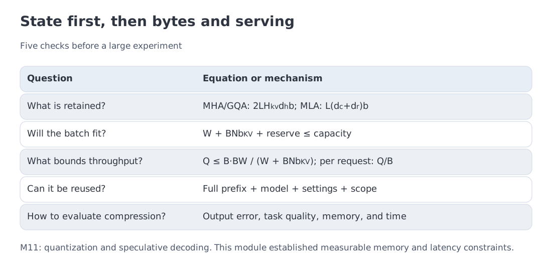 The module in one diagram: KV geometry, the bandwidth ceiling, batch knees, paged allocation, prefix reuse, tiered placement, phase disaggregation, and compression.
KV geometry comes first. For ordinary attention,
The teaching ladder is 2,560, 320, and 128 KiB/token for the MHA/GQA configurations and 68.625 KiB/token for the separate MLA geometry. A hybrid model requires an inventory of its actual stored state before any capacity calculation.
Context lowers the memory-bound ceiling. In the simplified model,
For the 8B bf16 scenario, batch-one throughput falls from 209.4 tok/s with no KV to 101.0 at 128K and 22.8 at 1M. These are arithmetic ceilings, not measurements of a particular engine.
Batching has a changing return. marks the scale at which aggregate KV traffic catches the weight payload. Longer context moves the knee toward smaller batches.
Memory management and state reduction are different jobs. PagedAttention reduces allocation waste and enables sharing. Prefix caching removes repeated prefill for exact common beginnings.
Storage tiers (reference). LMCache and Mooncake extend placement and reuse beyond one process or one memory tier. Prefill/decode disaggregation separates latency-sensitive decode from long prompt work at the cost of explicit KV transport.
Compression levers act on different quantities. Architectural methods change the base state, quantization changes bytes per coordinate, tiering changes location, and eviction changes which positions survive. They can be combined, but their quality and operational risks differ.
Primary sources
- MQA: Fast Transformer Decoding: One Write-Head is All You Need
- GQA: GQA: Training Generalized Multi-Query Transformer Models
- iteration-level scheduling / continuous batching: Orca, OSDI 2022
- PagedAttention and vLLM: Efficient Memory Management for Large Language Model Serving and vLLM stable documentation
- RadixAttention and SGLang: SGLang
- external and tiered KV: LMCache repository, LMCache/vLLM examples, and Mooncake, FAST 2025
- distributed orchestration: NVIDIA Dynamo 1.0 and NVIDIA CMX
- public caching contracts: OpenAI prompt caching, Anthropic prompt caching, Kimi K3, and vLLM’s Kimi K3 serving note
- hybrid state geometry: DeepSeek V4 technical report and vLLM’s DeepSeek V4 serving note
- eviction: StreamingLLM, H2O, SnapKV, reasoning benchmark, and structural-protection study
- quantization: KIVI, KVQuant, TurboQuant, and Google Research overview
Next. Module 11 studies quantization and speculative decoding: move fewer bytes per step, or validate several tokens in one target-model pass. Output-format constraints return in Module 18 with tools and agents.
Sources and service contracts checked on 11 October 2026. Teaching numbers are rebuilt from the local numerical contract; verify engine support and prices for the version used in an experiment.