Module 13. Supervised Fine-Tuning and Data Work
Modern LLMs · Module 13 lecture · revision October 11, 2026
What this module is about. Pretraining gives a model a remarkably broad next-token predictor. It does not, by itself, specify how a conversational system should represent roles, obey a system instruction, stop a turn, emit a tool call, or expose different parts of a structured response. Supervised fine-tuning (SFT) supplies demonstrations of the behavior we want.
The route. We follow the chain from a demonstration to the behavior it teaches. We will connect serialization, label construction, sequence packing, data curation, synthetic generation, reasoning demonstrations, tool-use traces, distillation, and LoRA. Four reproducible scenarios anchor the discussion: 21 supervised positions in a 56-token conversation; 24 examples packed into five 2,048-token containers; an explicit SFT compute estimate; and 13.63 million LoRA parameters in place of updating an entire 8.03B model.
Prerequisites. The tokenizer and special-token discussion from Module 2, the data and compute accounting from Module 9, and the quantization concepts from Module 11 are useful background. All definitions needed for the calculations are repeated here.
1. Why next-token prediction is not yet an assistant
Reading routes. For a first pass, follow §§1–6, read the interpretation of the cost calculation in §7, then continue through §§8–12 and the explanations of distillation and LoRA in §§15–16. The NumPy → PyTorch checks can wait; the surrounding prose supplies the concepts. On a second pass, reproduce the numerical scenarios and work through §§13–14 with the notebook. Sections 2, 8, 16.1 and 17 also provide a reference route for papers and checkpoint files.
We return here to an autoregressive Transformer after Module 12's diffusion models. SFT names a demonstration-based training stage, not an architecture. A diffusion model can learn from demonstrations using conditional denoising, but the next-token label shift developed below is specific to the autoregressive path.
A pretrained language model has spent its training budget minimizing a deceptively simple objective:
That objective rewards plausible continuation. It does not contain a separate term for respecting the boundary between a user turn and an assistant turn. It does not say that a JSON object must match a tool schema, that a refusal should be concise, or that the model should stop after answering.
This distinction matters because a continuation can be statistically reasonable and operationally wrong. After a line such as What is 2+2?, a web page may continue with another exercise rather than the answer. A base model that does the same is behaving consistently with pretraining, even though it is failing the product contract.
SFT changes the conditional behavior by training on deliberately constructed demonstrations. The learning rule is still next-token prediction, but the sequence now encodes roles, message boundaries, and an example of the desired response. In most assistant recipes, the loss is concentrated on assistant-generated positions, so the model is optimized to produce the response given the prompt rather than to reconstruct every token in the prompt.
SFT is best understood as behavioral adaptation. It can inject narrow facts or domain patterns, but it is not the most reliable mechanism for loading a large body of knowledge. Continued training modifies parameters, while retrieval and tools make information available in the response context. Reading an external document does not by itself store its facts in the weights. The choice depends on update frequency, source traceability, and the capability being taught; these approaches can be combined with SFT.
The practical work falls into four layers:
- representation: convert a conversation into the exact token grammar expected by the checkpoint;
- objective: decide which positions should contribute to the loss;
- systems: minimize padding and memory waste without allowing examples to leak into one another;
- data: choose demonstrations whose behavior is worth imitating.
The last layer usually dominates final quality, but the first three determine whether the data means what we think it means.
2. From instruction tuning to structured post-training
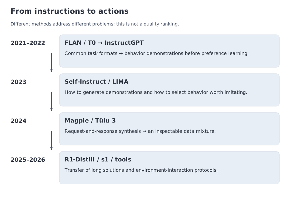 The trajectory from multitask instruction tuning to open alignment recipes, synthetic data, reasoning transfer, and structured tool-aware response formats.
Modern SFT grew out of several research programs rather than a single canonical recipe.
FLAN and T0 established the value of expressing many supervised tasks through natural-language instructions. They showed that instruction-tuned models could generalize to task formulations not seen verbatim during training. InstructGPT then placed SFT at the beginning of a larger alignment pipeline: demonstrations created a useful initial policy before reward modeling and reinforcement learning.
Open recipes accelerated in 2023. Self-Instruct used a language model to expand a seed collection of instructions. LIMA took a different path: only 1,000 carefully curated examples were used to fine-tune a 65B LLaMA model, producing surprisingly strong instruction-following behavior. That result made data selection a first-class research question.
The next wave focused on synthesis. Magpie observed that an aligned model can generate a user request when prompted only with the left side of its own chat template. The authors generated four million instructions and selected 300,000 high-quality instances. Tülu 3 provided a particularly transparent open post-training stack in which an SFT mixture feeds later preference learning and reinforcement learning with verifiable rewards (RLVR). A verifiable reward can come from executable tests; Module 14 explains how it drives learning.
Reasoning distillation became prominent in 2025. DeepSeek fine-tuned several smaller open models on roughly 800,000 curated samples produced through the DeepSeek-R1 pipeline. The s1 project explored the opposite end of the data scale, using only 1,000 selected reasoning examples for a 32B model.
Response formats also became more explicit. Tool calls, hidden or internal channels, final user-visible text, and role hierarchy can no longer be treated as informal punctuation conventions. OpenAI's Harmony format for gpt-oss is one example: it represents analysis, commentary, and final as distinct channels in the serialized response.
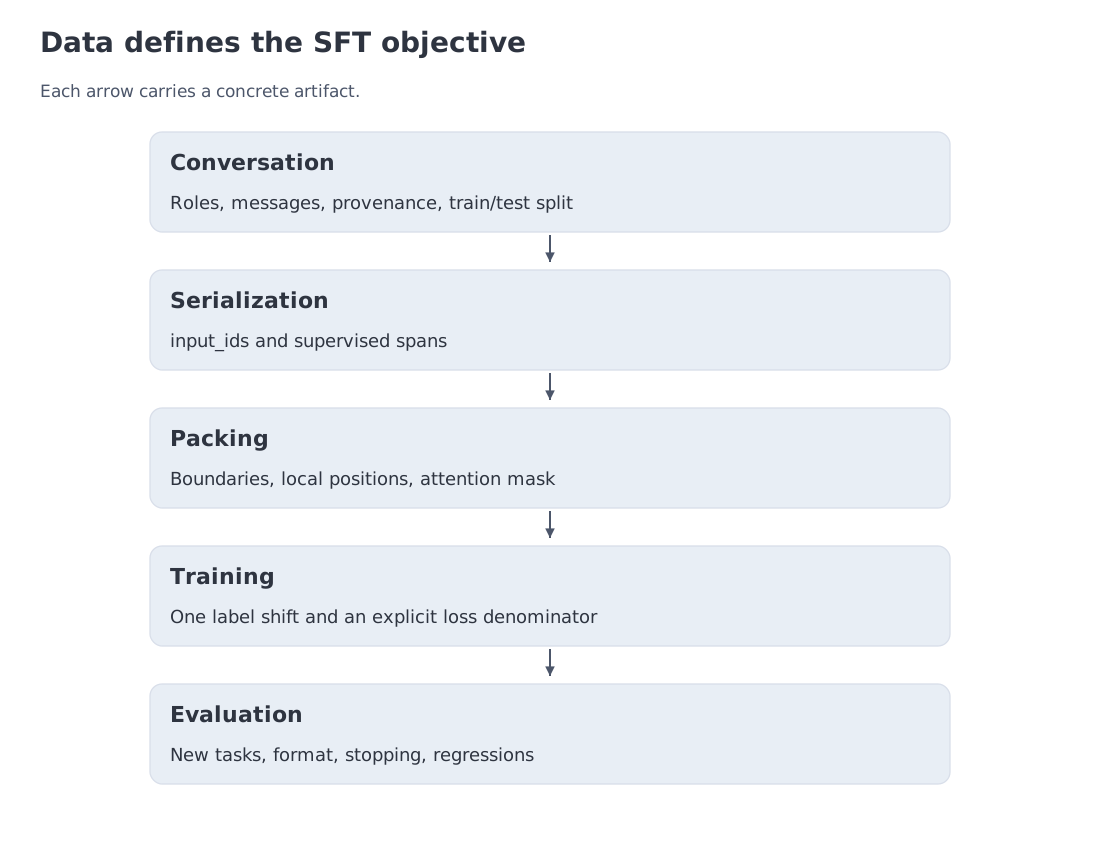 A complete SFT route: base checkpoint, tokenizer contract, curated demonstrations, packing and isolation, supervised labels, parameter update strategy, and behavioral evaluation.
3. Three older ideas hiding inside SFT
The current vocabulary is easier to navigate when we connect it to established machine-learning concepts.
Transfer learning
SFT follows the familiar pattern of broad pretraining followed by narrow adaptation. The expensive stage builds reusable representations; the cheaper stage specializes the model for a task distribution and an interaction protocol.
It is tempting to say that SFT changes only a superficial “behavior layer.” That metaphor is useful but not literal. In full fine-tuning, gradients may update parameters throughout the network. What makes the change behaviorally focused is the small dataset, modest learning rate, limited number of epochs, and narrow distribution of supervised examples.
Behavior cloning
A policy assigns probabilities to actions given a state . A demonstration dataset supplies state–action pairs, and behavior cloning maximizes the probability of those demonstrated actions:
For an autoregressive model, the state is the current dialogue prefix and the action is the next assistant token. This analogy exposes an important limitation: training states come from expert demonstrations, while deployment states are partly generated by the model itself. Once the model makes a mistake, subsequent prefixes may drift away from the demonstration distribution.
Preference optimization and RL can train on model-generated responses and therefore address part of this mismatch. They do not automatically eliminate hallucination or compounding error; the policy, data, reward, and evaluation environment still determine the outcome.
Further study. The relationship between SFT, behavior cloning, on-policy data, and rollout distributions is developed in the RL for LLM course.
Dataset design
SFT inherits every classical lesson about labels: coverage, disagreement, duplicates, leakage, and class imbalance. The object being labeled is richer, however. A response has factual content, format, style, length, refusal behavior, tool decisions, and implicit assumptions. The model learns all of them at once.
That is why curation is not a preliminary cleanup step. It is part of the model specification.
4. Chat templates are executable contracts
Training data is often stored as a list of messages, but the Transformer consumes a single token sequence. A chat template maps roles and message content into that sequence.
In the Hugging Face ecosystem, the template is commonly stored in tokenizer_config.json and rendered through tokenizer.apply_chat_template. It determines more than visual formatting. It specifies:
- role markers;
- turn boundaries;
- beginning and end tokens;
- the placement of a system or developer instruction;
- tool-call and tool-result syntax;
- stopping tokens;
- optional response channels.
Llama-family templates use role headers and an end-of-turn token such as <|eot_id|>. ChatML-like templates use markers such as <|im_start|> and <|im_end|>, but implementations diverge across model families. A model described as “ChatML-compatible” may still have different tool tokens, stop conditions, or reasoning markup.
Harmony makes channel structure explicit. A message has a role and content, while the response can be emitted through analysis, commentary, or final. Tool namespaces and structured constraints are represented by the format rather than reconstructed from ad hoc text parsing.
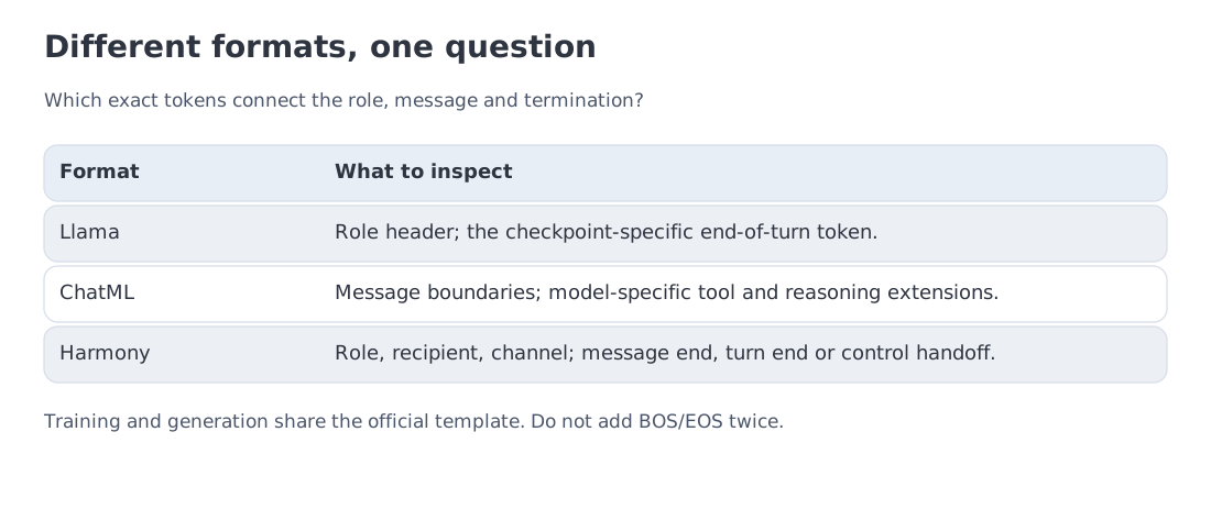 Several ways to serialize the same interaction: Llama role headers, ChatML-style delimiters, Harmony channels, and model-specific reasoning or tool tokens. The tokenizer contract is the source of truth.
A wrong template can produce a deceptively healthy training run. Loss decreases because the model learns the supplied sequence distribution, but deployment uses a different distribution. The safe workflow is simple: render examples with the official tokenizer, inspect token IDs around every boundary, and compare them with the model card and generation configuration.
5. Label masking: a 56-token example
Two masks serve different purposes. An attention mask controls which context a position may use; a loss mask chooses which predictions are scored. Removing prompt tokens from the loss does not remove their representations from the computation. Gradients from the answer can still flow through the processing of those prompt tokens.
Let be the stored tokens and let indicate that is a supervised target. Token-averaged training minimizes
Our labels[t] stores the target at its own position. We compare it with logits[t-1]; either the model or the caller performs that shift, exactly once. A batch with no active shifted targets has no defined mean loss and needs an explicit filtering or skip rule. The example below has 21 supervised tokens among 56 stored tokens. There are 55 next-token pairs after excluding the unpredicted BOS, of which 21 are scored.
The denominator also decides how examples are weighted. Pooling token losses gives longer answers more influence. Averaging each example's mean gives equal weight to examples. An answer with one loss of 2 and another with three losses of 1 produce a pooled mean of 1.25 but an example mean of 1.5. Both objectives are possible; gradient accumulation across microbatches must preserve whichever one was chosen.
Causal language modeling normally predicts the next token at every position. SFT often modifies the labels so that only assistant-generated tokens contribute directly to the cross-entropy loss.
PyTorch uses -100 as the conventional ignore_index. A system or user token remains in the input and affects the hidden state, but its label is ignored. This produces an assistant-only loss.
Assistant-only masking is common, not mandatory. Full-sequence loss may be appropriate in continued pretraining or in a deliberately chosen instruction-tuning recipe. The mask should express the objective rather than imitate a framework default.
Consider the frozen accounting scenario used throughout this module:
- one BOS token;
- three messages: system, user, assistant;
- five structural tokens per message;
- 12, 8, and 20 content tokens respectively.
The total sequence length is
If the supervised region contains 20 assistant-content tokens plus the assistant end-of-turn token, then
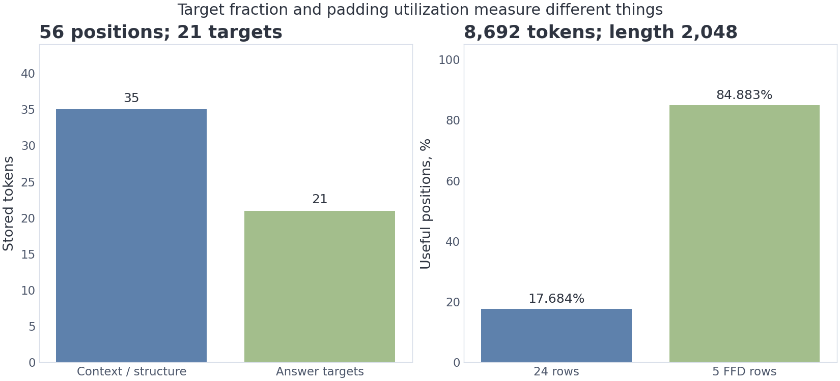 The left panel decomposes the 56-token dialogue and its 21 supervised positions. The right panel shows the packing scenario used in the next section.
The end-of-turn token is not cosmetic. It teaches the model where the demonstrated response ends. The exact token is model-specific, so <|eot_id|> should be read as part of this scenario rather than a universal constant.
Reasoning channels require a policy decision. If a reasoning trace is a target output, its tokens can be supervised. If a system has a private channel, the training pipeline may include, exclude, or separately weight it. That choice determines both behavior and disclosure; there is no single masking rule for all reasoning models.
NumPy → PyTorch · B20 — Assistant-only labels
A label contains the real token ID or -100; the boolean mask only selects positions that contribute to the loss.
import numpy as np
import torch
1. Explicit NumPy implementation
def numpy_assistant_labels(input_ids: np.ndarray, assistant_mask: np.ndarray, *, ignore_index: int = -100) -> np.ndarray:
    ids, mask = np.asarray(input_ids), np.asarray(assistant_mask)
    if ids.dtype != np.int64 or mask.dtype != np.bool_:
        raise TypeError("use int64 token IDs and a boolean assistant mask")
    if np.any(ids < 0):
        raise ValueError("input token IDs must be nonnegative")
    if ids.shape != mask.shape:
        raise ValueError("input_ids and assistant_mask must have identical shapes")
    return np.where(mask, ids, ignore_index).astype(np.int64)
The boolean mask is not the label itself. NumPy keeps the real token ID on assistant positions and writes ignore_index everywhere else.
2. The same mathematics as explicit PyTorch operations
def torch_assistant_labels(input_ids: torch.Tensor, assistant_mask: torch.Tensor, *, ignore_index: int = -100) -> torch.Tensor:
    if input_ids.dtype != torch.long or assistant_mask.dtype != torch.bool:
        raise TypeError("use torch.long token IDs and a boolean assistant mask")
    if input_ids.device != assistant_mask.device:
        raise ValueError("input IDs and mask must share a device")
    if torch.any(input_ids < 0):
        raise ValueError("input token IDs must be nonnegative")
    if input_ids.shape != assistant_mask.shape:
        raise ValueError("input_ids and assistant_mask must have identical shapes")
    labels = input_ids.clone()
    return labels.masked_fill(~assistant_mask.to(torch.bool), ignore_index)
Use nonnegative np.int64 / torch.long IDs and a boolean mask of the same shape; Torch inputs share a device. The result stores labels at their own positions. Align logits[..., :-1, :] with labels[..., 1:] exactly once before cross-entropy. A model that shifts internally must receive unshifted arrays. The loss function checks that active targets exist and belong to its vocabulary.
| Aspect | NumPy | PyTorch |
|---|---|---|
| Label value | real token ID | same ID |
| Ignore | np.where | masked_fill |
| Shape | must match the mask | validated before the operation |
| Autograd | not applicable to integer labels | loss differentiates logits, not labels |
Executable parity and edge-case check
ids_np = np.array([10,11,12,13,14,15]); mask_np = np.array([0,0,0,1,1,1], dtype=bool)
np_labels = numpy_assistant_labels(ids_np, mask_np); t_labels = torch_assistant_labels(torch.tensor(ids_np), torch.tensor(mask_np))
np.testing.assert_array_equal(np_labels, t_labels.numpy()); assert np_labels.tolist() == [-100,-100,-100,13,14,15]
# Labels are stored at their own positions. Shift them once for explicit CE.
scores = torch.zeros((len(ids_np), 20), dtype=torch.float64, requires_grad=True)
loss = torch.nn.functional.cross_entropy(scores[:-1], t_labels[1:], ignore_index=-100)
torch.testing.assert_close(loss, torch.log(torch.tensor(20.,dtype=torch.float64)))
loss.backward()
assert torch.count_nonzero(scores.grad[-1]) == 0
assert torch.count_nonzero(scores.grad[:2]) == 0
for ids_bad, mask_bad in [(ids_np.astype(float),mask_np),
                           (ids_np,mask_np.astype(int)),
                           (np.array([-1,1]),np.array([False,True]))]:
    for run in (lambda: numpy_assistant_labels(ids_bad,mask_bad),
                lambda: torch_assistant_labels(torch.tensor(ids_bad),torch.tensor(mask_bad))):
        try:
            run()
        except (TypeError,ValueError):
            pass
        else:
            raise AssertionError("invalid label input was accepted")
print("B20 assistant labels: PASS")
Complete executable file: m13_sft_bridges.py
6. Packing variable-length examples safely
Padding is often the first major efficiency loss in SFT. When a 300-token example is padded to 2,048 tokens, most positions carry no learning signal. Sequence packing combines several examples in one fixed-length container.
The module's deterministic length list contains 24 examples totaling 8,692 tokens. Padding every example independently to 2,048 tokens yields
useful positions.
First-Fit Decreasing sorts examples by length and places each one in the first container with enough remaining capacity. For this list, the five resulting container loads are 2,045, 2,017, 2,044, 2,047, and 539. Utilization becomes
The number of fixed-length rows falls from 24 to five, a factor of 4.8. That factor is not a throughput guarantee. Real speed depends on kernel support, batch shape, attention implementation, device occupancy, and the distribution of sequence lengths. The calculation quantifies removed padding.
Correctness is the harder part. If two examples are merely concatenated under an ordinary causal mask, later examples can attend to earlier ones. An EOS separator marks a boundary semantically but does not remove those attention edges.
A correct packed implementation uses either:
- a block-diagonal causal attention mask; or
- a variable-length attention kernel supplied with sequence boundaries such as
cu_seq_lens.
Resetting position_ids may be useful, but it is not an isolation mechanism by itself. The notebook includes an explicit negative test for cross-example leakage because visual inspection of the token buffer is not sufficient.
Attention isolation is only half the boundary contract. A global label shift pairs the final logit of example A with the first token of example B. Blocking attention cannot repair that target pair. The first label of each independent segment must therefore be ignored. BOS already satisfies this rule in our teaching template; the packer enforces it even when given a different source example.
A useful regression test compares separate and packed execution with dropout disabled: the same tokens and local positions should produce matching logits, summed loss and gradients. The training lab runs this test. Padding needs its own handling: a naive softmax over a fully forbidden row is undefined, so an implementation must omit such queries or rely on a kernel whose behavior for them has been checked.
NumPy → PyTorch · B21 — Isolating packed dialogues
segment_ids identify independent dialogues, position_ids reset per segment, and the boolean mask allows only causal attention inside the same segment.
import numpy as np
import torch
1. Explicit NumPy implementation
def numpy_segment_position_ids(segment_ids: np.ndarray, *, padding_id: int = -1) -> np.ndarray:
    segments = np.asarray(segment_ids)
    if segments.ndim not in (1, 2):
        raise ValueError("segment_ids must be [T] or [B,T]")
    batch = segments[None, :] if segments.ndim == 1 else segments
    positions = np.zeros_like(batch, dtype=np.int64)
    for row in range(batch.shape[0]):
        for col in range(1, batch.shape[1]):
            current, previous = batch[row, col], batch[row, col - 1]
            if current != padding_id and current == previous:
                positions[row, col] = positions[row, col - 1] + 1
    return positions[0] if segments.ndim == 1 else positions

def numpy_block_causal_mask(segment_ids: np.ndarray, *, padding_id: int = -1) -> np.ndarray:
    segments = np.asarray(segment_ids)
    if segments.ndim not in (1, 2):
        raise ValueError("segment_ids must be [T] or [B,T]")
    batch = segments[None, :] if segments.ndim == 1 else segments
    t = batch.shape[-1]
    boundaries = np.ones_like(batch, dtype=bool)
    if t > 1:
        boundaries[:, 1:] = batch[:, 1:] != batch[:, :-1]
    run_ids = np.cumsum(boundaries, axis=-1)
    same = run_ids[:, :, None] == run_ids[:, None, :]
    valid = (batch[:, :, None] != padding_id) & (batch[:, None, :] != padding_id)
    causal = np.arange(t)[None, None, :] <= np.arange(t)[None, :, None]
    out = same & valid & causal
    return out[0] if segments.ndim == 1 else out
NumPy first numbers contiguous runs, then permits attention only within one run and only causally. position_ids reset at every boundary.
2. The same mathematics as explicit PyTorch operations
def torch_segment_position_ids(segment_ids: torch.Tensor, *, padding_id: int = -1) -> torch.Tensor:
    if segment_ids.ndim not in (1, 2):
        raise ValueError("segment_ids must be [T] or [B,T]")
    batch = segment_ids.unsqueeze(0) if segment_ids.ndim == 1 else segment_ids
    positions = torch.zeros_like(batch, dtype=torch.long)
    for col in range(1, batch.shape[-1]):
        continues = (batch[:, col] != padding_id) & (batch[:, col] == batch[:, col - 1])
        positions[:, col] = torch.where(continues, positions[:, col - 1] + 1, 0)
    return positions[0] if segment_ids.ndim == 1 else positions

def torch_block_causal_mask(segment_ids: torch.Tensor, *, padding_id: int = -1) -> torch.Tensor:
    if segment_ids.ndim not in (1, 2):
        raise ValueError("segment_ids must be [T] or [B,T]")
    batch = segment_ids.unsqueeze(0) if segment_ids.ndim == 1 else segment_ids
    t = batch.shape[-1]
    boundaries = torch.ones_like(batch, dtype=torch.bool)
    if t > 1:
        boundaries[:, 1:] = batch[:, 1:] != batch[:, :-1]
    run_ids = boundaries.to(torch.long).cumsum(dim=-1)
    same = run_ids[:, :, None] == run_ids[:, None, :]
    valid = (batch[:, :, None] != padding_id) & (batch[:, None, :] != padding_id)
    idx = torch.arange(t, device=batch.device)
    causal = idx[None, None, :] <= idx[None, :, None]
    out = same & valid & causal
    return out[0] if segment_ids.ndim == 1 else out
PyTorch builds the same run_ids, mask, and positions on the tensor device. Contiguous runs—not only numeric labels—matter because a segment label may reappear later.
| Aspect | NumPy | PyTorch |
|---|---|---|
| Boundary | change in adjacent segment_id | same boolean test |
| Positions | loop over T | loop over positions on the input device |
| Isolation | same_run & causal & valid | same boolean mask |
| Padding | segment -1 is forbidden | same contract |
| Regression | change A; B stays fixed | SDPA checks B logits/output |
Executable parity and edge-case check
segments_np = np.array([0,0,0,1,1,1,-1]); np_pos = numpy_segment_position_ids(segments_np); np_mask = numpy_block_causal_mask(segments_np)
t_segments = torch.tensor(segments_np); t_pos = torch_segment_position_ids(t_segments); t_mask = torch_block_causal_mask(t_segments)
np.testing.assert_array_equal(np_pos, t_pos.numpy()); np.testing.assert_array_equal(np_mask, t_mask.numpy())
rng = np.random.default_rng(21); x = torch.tensor(rng.standard_normal((1,1,7,4)), dtype=torch.float64); mask = t_mask[None,None]
out_a = torch.nn.functional.scaled_dot_product_attention(x, x, x, attn_mask=mask)
x_changed = x.clone(); x_changed[..., :3, :] += 1000
out_b = torch.nn.functional.scaled_dot_product_attention(x_changed, x_changed, x_changed, attn_mask=mask)
torch.testing.assert_close(out_a[..., 3:6, :], out_b[..., 3:6, :], rtol=0, atol=0)
repeated = np.array([0,0,1,1,0,0])
np.testing.assert_array_equal(numpy_segment_position_ids(repeated), [0,1,0,1,0,1])
repeat_mask = numpy_block_causal_mask(repeated)
assert not repeat_mask[4,0] and repeat_mask[5,4]
print("B21 packed isolation: PASS")
Complete executable file: m13_sft_bridges.py
7. Compute accounting and hyperparameters
SFT is cheap relative to pretraining, but “cheap” should be supported by a stated scenario.
Take an 8.03B-parameter model, 200,000 examples, 1,200 tokens per example on average, and three epochs. One epoch contains
Using the training approximation from Module 9,
Here counts every processed token, including the prompt. Assistant-only supervision does not make the forward processing of that prompt disappear, so multiplying compute by 21/56 would be incorrect. The rule approximates dense-model forward and backward work; it is not a rigorous lower bound and changes when parameters are frozen. Model FLOP utilization (MFU) compares useful model work with peak FLOP/s. The assumed 40% is an input to this scenario, not a measured efficiency.
The comparison pretraining scenario uses 15 trillion tokens and therefore costs FLOP for the same parameter count. The ratio is approximately 20,833. This is a ratio between two declared workloads, not a property of SFT in general.
At 990 TFLOP/s peak and an assumed model FLOP utilization of 40%, the arithmetic wall-clock estimate is
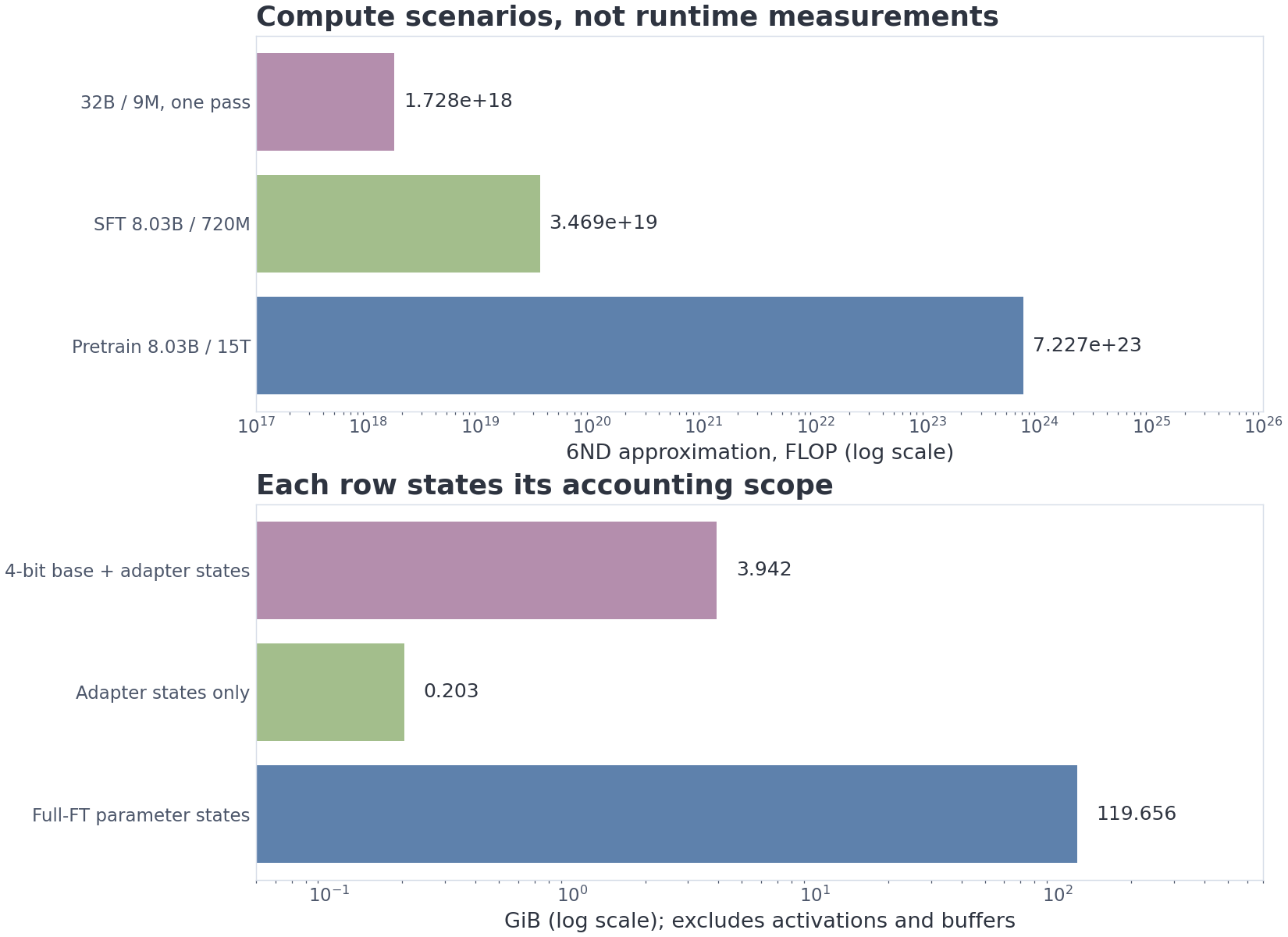 Orders of magnitude for the pretraining, SFT, and one-pass s1 scenarios, together with parameter-state memory for full fine-tuning and LoRA.
The estimate is useful because it changes experimental strategy. If the adaptation run is affordable, data ablations, template checks, and held-out behavioral evaluations deserve more attention than a single monolithic run.
Reasonable starting ranges are not universal defaults:
| Quantity | Initial search region |
|---|---|
| Epochs | 1–3, with held-out and behavioral monitoring |
| Full-FT learning rate | roughly to |
| LoRA learning rate | often to |
| LoRA rank | 8–64, depending on the adaptation |
| Effective batch | tune in tokens, not examples alone |
| Maximum length | match the target distribution |
| Schedule | a smooth decay with a short warmup is common |
| Gradient clipping | a safeguard, not a substitute for diagnosis |
Training loss is only one signal. A useful run also tracks skill-specific validation, format validity, regressions on general capability, and human inspection of generated outputs.
8. Organizing SFT data by capability
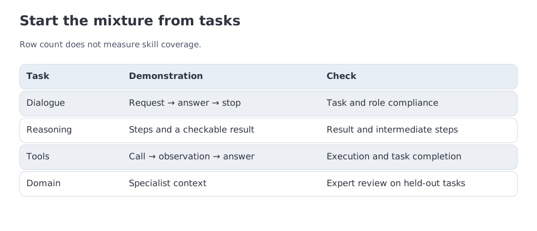 Data organized by function: general instruction following, reasoning demonstrations, tool trajectories, and domain or style adaptation.
A dataset name is not a training strategy. A production mixture usually combines several functional categories.
General instruction following
This category includes conversational and multitask data such as OpenAssistant, UltraChat, WildChat-derived sets, FLAN-derived tasks, code, mathematics, multilingual examples, and safety or non-compliance demonstrations.
The Tülu 3 SFT Mixture is a useful open reference because it documents a mixture reported as 939,344 examples in its card, the contributing subsets, and licensing caveats. Its value is not that 939,344 is a magic number; it is that the composition is inspectable.
The mixture also illustrates why a card and a file are different evidence. At the check date, the Tülu 3 card reports 939,344 samples while the viewer counts 939,343 rows. A reproduction should pin a revision and count the loaded records. The collection license does not replace component licenses; the card explicitly flags non-commercial portions. We use it as a documented mixture example, not as the embedded data for this module's exercises.
Reasoning demonstrations
These examples pair a problem with a longer solution and a final answer. DeepSeek reports that its R1 distillation stage used about 800,000 curated examples—roughly 600,000 reasoning-related and 200,000 non-reasoning samples. The distilled checkpoints were released, but those 800,000 examples should not be described as an open dataset unless a separate release provides them.
Open reasoning datasets such as AM-DeepSeek-R1-Distilled-1.4M provide another route, but they require the same checks as any synthetic corpus: benchmark contamination, teacher artifacts, verifier quality, and duplicate solution patterns.
Tool trajectories
Tool data includes function definitions, user requests, calls, tool results, and potentially multiple dependent steps. xLAM-function-calling-60k supplies 60,000 single-turn examples. ToolACE builds synthetic conversations over a large API pool and applies rule-based plus model-based verification. Multi-turn agent training needs trajectories in which each action depends on the observation returned by the environment.
Domain and style adaptation
A small expert dataset can be more valuable than a much larger generic mixture when the target behavior is narrow: legal drafting conventions, a customer-support policy, a product ontology, or a specific response style. The key question is whether the demonstrations cover the decisions the model must make, not whether the row count resembles another project.
9. Reading LIMA correctly
Split by source family before producing derived data. If a teacher paraphrases one problem five times, a random row split may put four versions in training and the fifth in validation. The strings differ, but the underlying task has already been exposed. Keep an original problem, its revisions and all synthetic answers in one split. The same reasoning applies to related documents, conversations from one user, or tests from one software project.
LIMA fine-tuned a 65B LLaMA model on only 1,000 curated prompt-response pairs, without reinforcement learning or preference modeling. The model learned strong instruction-following behavior and was competitive with much more expensive contemporary systems in a controlled human study.
The paper's Superficial Alignment Hypothesis proposes that pretraining learns most knowledge and capability, while a relatively small amount of alignment data teaches the model which subdistribution of behavior to expose.
The finding is important, but it is easy to overgeneralize. LIMA does not prove that every model, language, safety requirement, tool protocol, and professional domain can be covered with 1,000 examples. Its result depends on a large base model, carefully selected demonstrations, and the evaluation setting.
A durable lesson is that demonstrations are multidimensional labels. They specify:
- correctness;
- relevance;
- structure;
- tone;
- degree of detail;
- uncertainty handling;
- refusal behavior;
- stopping behavior.
Poor examples push all of those dimensions in the wrong direction. Data cleaning should therefore include executable checks where possible, semantic deduplication, benchmark-contamination scans, length and difficulty analysis, teacher-style diagnostics, and stratified human review.
The objective is not to maximize dataset size. It is to make the empirical behavior distribution match the intended model contract.
10. Synthetic data as a search-and-filter system
Synthetic generation becomes much more reliable when treated as candidate search rather than automatic labeling.
Self-Instruct expands a seed collection. Evol-Instruct modifies examples to increase difficulty. Magpie prompts an aligned model with only the left side of the user-turn template and lets the model synthesize both the request and the response.
A robust pipeline records more than the final text:
- task source and transformation history;
- teacher model and exact version;
- sampling parameters;
- candidate set;
- verifier decisions;
- deduplication and contamination results;
- the reason a sample was retained.
For verifiable tasks, best-of- makes the economics explicit. Suppose one candidate passes with probability and candidates are independent. The probability that at least one of candidates passes is
| At least one pass | Expected yield per generation if at most one sample is kept | |
|---|---|---|
| 1 | 0.3000 | 0.3000 |
| 4 | 0.7599 | 0.1900 |
| 8 | 0.9424 | 0.1178 |
| 16 | 0.9967 | 0.0623 |
Coverage saturates while generation cost continues to grow. Dependence can change coverage in either direction; pairwise correlations alone do not determine it. If candidates repeatedly share the same failure, additional attempts may add little coverage. Improving the task prompt, choosing a better teacher, or inserting an intermediate verifier can be more valuable than increasing .
Now consider a separate verifier-quality scenario. Let be the probability that a candidate is actually correct, the fraction of correct candidates accepted, and the fraction of incorrect candidates accepted. The pass rate and precision are
With , , and , the accepted mass is . Its precision is : roughly one in five accepted candidates is wrong. This scenario has , whereas the coverage table assumed 0.3. More candidates cannot make an imperfect filter certify correctness.
The table's final column measures retained examples per generation when at most one answer is kept. It divides coverage by the generations paid for; it does not estimate the correctness of the selected answer.
Second pass: pairwise correlation does not determine coverage
Take three candidates and assign their success count the probabilities . Conditional on , choose successful positions uniformly. Every candidate then has success probability . Each pair succeeds jointly with probability , so pairwise correlations are positive. Yet coverage is 0.9, above the independent value . The complete joint law matters. At the other extreme, perfectly identical outcomes leave coverage unchanged as candidates are added. The notebook checks both cases.
Connection to RL systems. Candidate sampling, verifiable filtering, and selected/rejected outputs reappear in preference optimization and RLVR. The RL for LLM course develops those pipelines in detail.
11. Reasoning demonstrations and the s1 compute scenario
A reasoning dataset supervises a sequence of intermediate steps rather than only the final answer. The student may learn useful decomposition patterns, checking behavior, and output structure—but it also inherits the teacher's mistakes, verbosity, and stylistic artifacts.
The DeepSeek-R1 report provides a clear empirical reference. The authors fine-tuned smaller Qwen and Llama models on about 800,000 curated examples. Under their evaluation protocol, DeepSeek-R1-Distill-Qwen-7B scored 55.5% pass@1 on AIME 2024. The 32B model scored 72.6% on AIME 2024 and 94.3% on MATH-500. These are author-reported benchmark results, not architecture-independent guarantees.
The s1 project explored data efficiency. It selected 1,000 questions and reasoning traces, fine-tuned Qwen2.5-32B-Instruct for five epochs, and reported 26 minutes of training on 16 H100 GPUs. The paper also introduced budget forcing: when the model attempts to terminate its reasoning, appending Wait can extend the trajectory. In the reported experiment, AIME 2024 accuracy increased from 50% to 57%.
The module's compute calculation answers a narrower question. For 1,000 traces averaging 9,000 tokens, one pass contains nine million tokens:
At eight 990-TFLOP/s accelerators and an assumed MFU of 40%, that is 9.09 minutes.
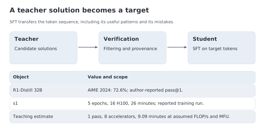 Reasoning transfer from a teacher to a student, with author-reported DeepSeek-R1-Distill results and a separate one-pass arithmetic estimate for the module's s1-like scenario.
The 9.09-minute value is not a reproduction of s1. It represents one epoch under stated throughput assumptions. The original run used five epochs, 16 devices, FSDP, and its own implementation. Comparing the figures without matching epochs and realized utilization would be misleading.
Long reasoning traces also change the systems profile:
- activation memory grows;
- length variance affects packing;
- incorrect intermediate steps become supervised targets;
- benchmark leakage becomes easier;
- the boundary between user-visible rationale and private model state must be specified explicitly.
SFT can transfer reasoning patterns efficiently. It does not certify that the transferred process is faithful, minimal, or robust.
12. Teaching a model to use tools
Function calling is a policy problem expressed through structured text. A model must decide whether a tool is needed, choose one from the available schema, populate arguments, interpret the returned observation, and decide what to do next.
A training trajectory therefore contains two distinct kinds of machine-readable content:
- an assistant action, such as a tool call, which is normally supervised;
- a tool observation, generated by the external environment, which is normally included as context but masked from the language-model loss.
In this recipe, tool observations supply evidence for the next assistant action. Masking them expresses that objective; other training schemes can model observations deliberately, provided that execution still supplies the real result at inference.
A useful curriculum covers at least five decisions:
- whether to call any tool;
- which tool is relevant;
- how to satisfy the schema exactly;
- how to handle missing data or execution failure;
- whether to issue another call or return a final answer.
xLAM-function-calling-60k is a large single-turn seed resource. ToolACE uses a broad API pool and dual verification. Multi-turn datasets add stateful dependencies and error recovery. Evaluation should separate syntax, executability, relevance detection, parallel calls, and task completion instead of collapsing everything into one score.
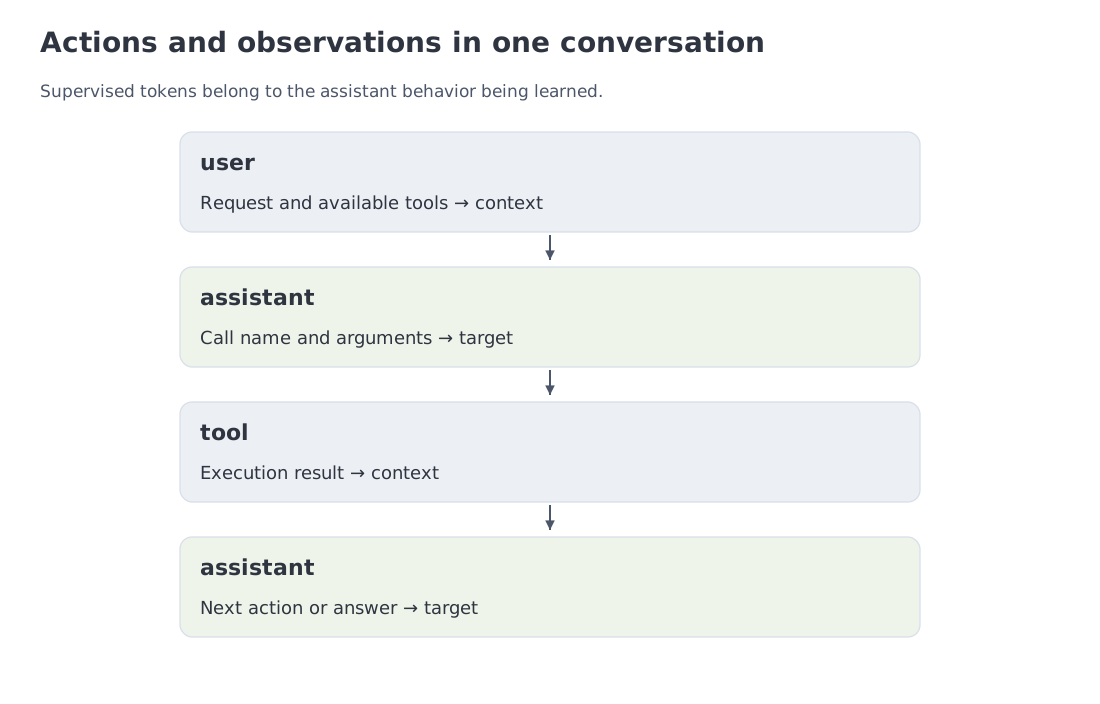 A tool-use trajectory separates the supervised assistant action from the environment observation, then continues until the model can answer or needs clarification.
The Berkeley Function-Calling Leaderboard has evolved from single-call syntax tests toward multi-turn and agentic scenarios in BFCL V4. That evolution is a useful warning: a model can format one correct JSON call and still fail at tool use as a sequential decision problem.
13. Level-one code: labels and traceable bins
The following code exposes the two structures that trainers often hide: target token IDs and the membership of each packed container.
import numpy as np

IGNORE_INDEX = -100

def build_sft_example(messages, special_ids):
    """Build input_ids and labels; supervise assistant content and EOT."""
    role_id = {
        "system": special_ids["role_system"],
        "user": special_ids["role_user"],
        "assistant": special_ids["role_assistant"],
        "tool": special_ids["role_tool"],
    }
    input_ids = [special_ids["bos"]]
    labels = [IGNORE_INDEX]

    for message in messages:
        header = [
            special_ids["start_header"],
            role_id[message["role"]],
            special_ids["end_header"],
            special_ids["newline"],
        ]
        body = [*message["token_ids"], special_ids["eot"]]

        input_ids.extend(header + body)
        labels.extend([IGNORE_INDEX] * len(header))
        labels.extend(
            body
            if message["role"] == "assistant"
            else [IGNORE_INDEX] * len(body)
        )

    return np.asarray(input_ids), np.asarray(labels)

def first_fit_decreasing(lengths, max_length=2048):
    """Keep original example indices in every First-Fit Decreasing bin."""
    if not isinstance(max_length, int) or isinstance(max_length, bool) or max_length <= 0:
        raise ValueError("max_length must be a positive integer")
    if any(not isinstance(n, (int, np.integer)) or isinstance(n, (bool, np.bool_)) for n in lengths):
        raise ValueError("lengths must be integers")
    bins = []
    for index in sorted(range(len(lengths)), key=lambda i: (-lengths[i], i)):
        length = lengths[index]
        if length <= 0 or length > max_length:
            raise ValueError("invalid sequence length")

        for bucket in bins:
            if bucket["used"] + length <= max_length:
                bucket["indices"].append(index)
                bucket["used"] += length
                break
        else:
            bins.append({"indices": [index], "used": length})

    return bins

def lora_params(d=4096, d_kv=1024, layers=32, rank=16):
    """Count q/k/v/o LoRA parameters for a GQA transformer."""
    per_layer = rank * (
        (d + d) + (d + d_kv) + (d + d_kv) + (d + d)
    )
    return per_layer * layers
The labels contain actual target token IDs. A boolean “train here” mask is not enough for a causal language-model loss. The packing function preserves original indices so the downstream pipeline can construct segment boundaries and identify the source of a failing sample.
15. Distillation channels
“Distillation” can mean several different supervision signals.
Hard targets
The teacher generates a response and the student trains on that response with ordinary cross-entropy. This works through an API and does not require teacher logits. It is also lossy: the student sees one sampled path, not the teacher's uncertainty over alternatives.
Hard-target distillation benefits from candidate diversity, executable verification, and careful metadata. A polished response from a powerful model is not automatically a trustworthy label.
Soft targets
Classical knowledge distillation trains the student to match a softened teacher distribution:
Temperature divides the logits before softmax, and sets the distillation weight. The KL direction is teacher-to-student: it penalizes the student for assigning little probability to events supported by the teacher. Multiplying by compensates for a change in gradient scale caused by softening; it does not make all temperatures equivalent. A softer distribution exposes relative preferences among alternatives, while and remain experimental choices.
For discrete distributions, over shared events, here tokens. A zero contributes zero; positive with zero gives infinite divergence. Matching distributions gives zero, and reversing the arguments generally changes the value. The objective requires teacher probabilities, available either directly or through logits. Tokenizer mismatch complicates the objective because the two models may not define probabilities over the same token events.
Further study. Cross-entropy, KL divergence, temperature, and the information content of a full distribution are covered in depth in Information Theory for ML.
Multiple teachers
A pipeline can route domains to specialized teachers, sample several teachers and select with a verifier, or combine distributions when compatible logits are available. Multiple teachers expand coverage, but they also introduce inconsistent style, policy, licensing, and calibration.
The engineering decision begins with the signal that is actually accessible. An API that returns only text supports hard targets. Full teacher probabilities or logits can support soft targets over compatible events; a truncated top-logprobs list does not by itself supply the complete vocabulary distribution. A verifiable task often benefits more from a strong checker than from an additional teacher.
16. LoRA and a concrete parameter count
Parameter-efficient fine-tuning (PEFT) updates a restricted parameter set. To make the memory calculation unambiguous, allocate 16 bytes per trainable parameter: 2 for its bf16 weight, 2 for its gradient, 4 for an fp32 master copy, and 4 for each of Adam's two moments. Implementations can store these objects differently. The adapter weight is already included in these 16 bytes.
Full fine-tuning stores trainable weights, gradients, and optimizer state for every updated parameter. Under the module's 16-byte-per-parameter accounting, an 8.03B model requires
for parameter-related training state alone.
Low-Rank Adaptation (LoRA) freezes the base matrix and learns
with and . The chosen scale controls the update through the multiplier . The adapter uses parameters for one target matrix.
Rank bounds the rank of the update , not of the complete matrix . Initializing one factor randomly and the other to zero preserves the starting model while allowing learning to begin. Initializing both to zero can leave both gradients zero. Frozen weights need no weight-gradient update, but backward propagation through them can still be needed to reach earlier adapters. Parameter savings therefore do not translate directly into the same FLOP savings.
For a 32-layer GQA model with , , rank 16, and adapters on q/k/v/o, the total is
or 0.1698% of the 8.03B base. At 16 bytes of training state per adapter parameter, that is 208 MiB. Dividing the full-state estimate by the adapter-state estimate gives approximately 589.
The ratio is deliberately narrow: it compares parameter-related state under one accounting convention. It is not a 589-fold reduction in total GPU memory.
QLoRA stores the frozen base in 4-bit form while backpropagating into LoRA adapters. The simplified floor in this module is:
- 3.739 GiB raw 4-bit base payload;
- 208 MiB adapter training state, including 26 MiB of bf16 adapter weights;
- 3.942 GiB total parameter-state floor.
Quantization scales, activations, temporary dequantization buffers, allocator overhead, and distributed-training metadata raise the real requirement.
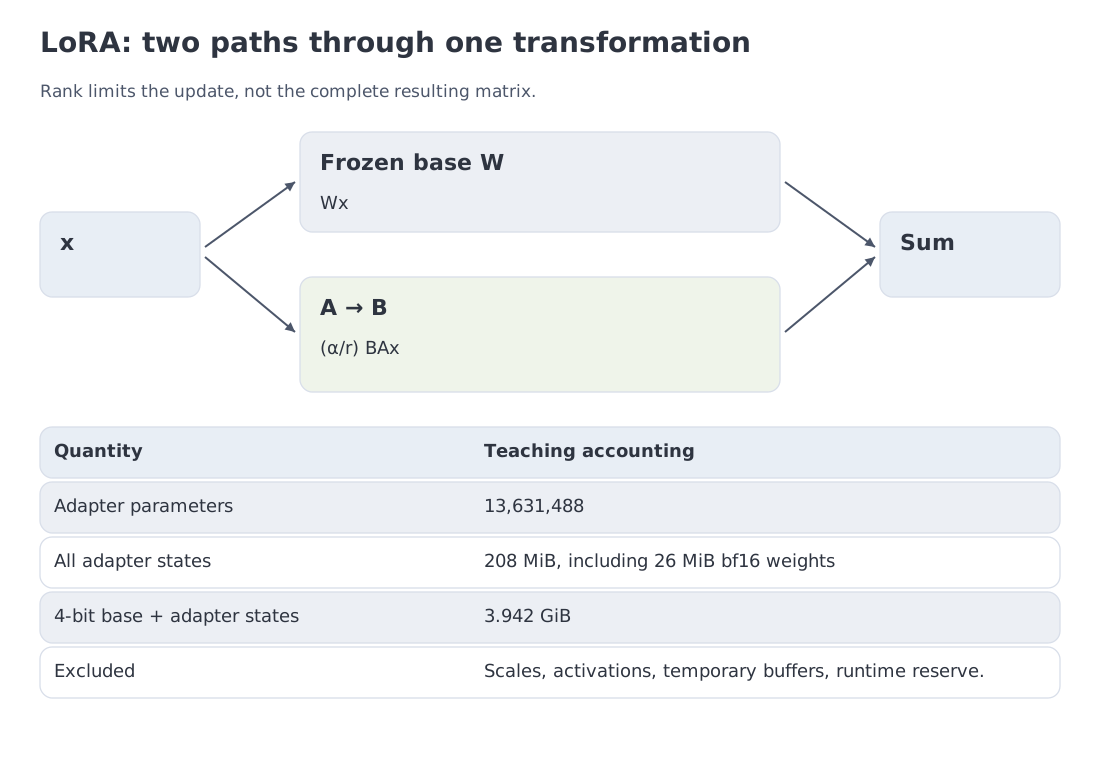 The low-rank update, the 13.63M-parameter calculation, and the boundary between parameter-state accounting and complete training memory.
LoRA is a strong baseline, not a theorem of equivalence to full fine-tuning. Rank, target modules, quantization, data scale, and the depth of the desired distribution shift determine the gap.
16.1. Tinker and Inkling: control without owning the cluster
Thinking Machines released Inkling in July 2026 as an open-weight MoE model with 975B total and 41B active parameters. Its Tinker platform exposes a managed training API built around operations such as forward_backward, optim_step, sample, and state saving.
This interface separates algorithm design from distributed execution. A user can define an SFT, LoRA, distillation, or RL loop while the service handles the underlying cluster.
The arrangement is useful for clarifying what “open” means:
- Are the model weights downloadable?
- Can the user implement a custom training objective?
- Is the distributed execution stack itself reproducible?
Inkling answers the first question positively. Tinker offers substantial control over the second. The third remains a managed-service boundary.
17. Reconstructing an SFT recipe from a checkpoint
A checkpoint directory often reveals more than its headline model card.
Tokenizer files. Inspect chat_template, added tokens, special-token maps, and stop IDs. Render actual conversations rather than inferring the format from one token name.
Three library details deserve a literal token-level check. A complete training conversation normally does not need an empty next-assistant header. If a template is first rendered to text and then tokenized, special tokens must not be added a second time. Finally, the assistant mask must come from valid spans in that actual template: TRL's assistant-only mode needs supported generation regions, commonly marked by Jinja generation blocks. Check these conventions against the installed library and official tokenizer, then inspect several serialized examples.
Adapter configuration. adapter_config.json may expose r, lora_alpha, target modules, dropout, DoRA flags, and the expected base model. These fields are enough to reproduce the parameter count for standard transformer projections.
Generation configuration. Stop sequences and decoding defaults describe deployment behavior, but they do not prove how the model was trained.
Model card and data statement. Look for source datasets, licenses, filtering, epoch count, context length, evaluation harness, and contamination checks. Published weights without a data recipe are useful, but not fully reproducible.
A disciplined inspection sequence is:
- render the official template;
- identify supervised roles and termination tokens;
- compute adapter size;
- audit data sources and licenses;
- reproduce at least one evaluation subset;
- only then interpret aggregate benchmark claims.
20. Key takeaways and sources
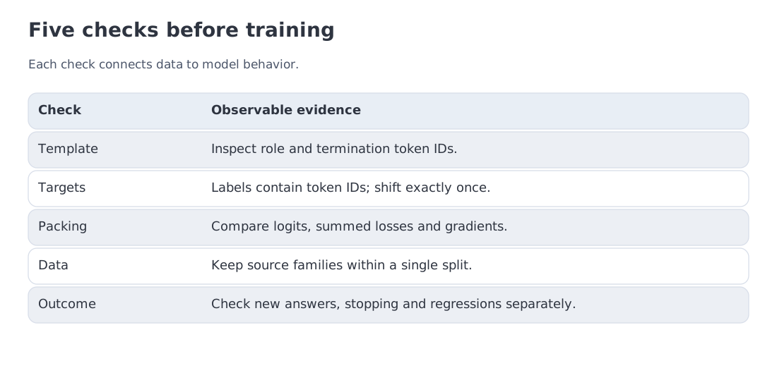 A compact map of the module: template contract, supervised positions, safe packing, compute, curation, synthesis, reasoning and tool demonstrations, distillation, and LoRA.
For the autoregressive model studied here, SFT remains next-token training, but the serialized protocol, target mask, and demonstration distribution turn it into behavioral adaptation.
- A chat template is part of the checkpoint contract.
- Assistant-only loss is a design choice that should be verified token by token.
- Packing removes padding only when examples remain attention-isolated.
- The module's compute ratios are scenario-specific arithmetic, not universal constants.
- LIMA argues for curation and coverage, not for a fixed minimal dataset size.
- Synthetic data is strongest when generation is paired with provenance and verification.
- Reasoning traces transfer strategies and artifacts together.
- Tool use requires action selection, schema compliance, observation handling, and stopping.
- LoRA changes parameter-state economics dramatically, but complete memory accounting remains broader.
Primary references:
Next: Module 14 moves from demonstrations to preferences and rewards. SFT supplies the initial policy and response grammar; DPO, RLHF, and RLVR will use comparative labels and rewards. DPO can work with a fixed pair dataset, while reinforcement learning usually refreshes model-generated samples.
Editorial and source check: October 11, 2026. Format, dataset, and service claims were checked against primary sources. Numerical scenarios are reproduced by local code; benchmark results retain the attribution and protocol of their original authors.