Module 15. Information Geometry: Fisher, Natural Gradient, and Distribution Flows
How to read this module. This is the final bonus module of the course. The main route is §§15.1–15.8: why ordinary gradient descent depends on coordinates, how Fisher information defines the local geometry of distributions, where the natural gradient comes from, which curvature approximations are actually used in deep networks, how this geometry appears in TRPO, PPO, and RLHF, and why moving probability mass requires a different geometry—Wasserstein geometry. §15.9 is a mathematical deepening on α-geometry, exact geodesics, and Chentsov’s theorem. It can be saved for a second pass.
15.1. What Does a “Small Step” Mean for a Probabilistic Model?
An optimizer moves parameters. What we usually care about, however, is not the parameter vector itself but the distribution, function, or policy that it represents.
Start with the smallest possible probabilistic model: a Bernoulli distribution. We may parameterize the event probability directly as
or through a logit
These are two coordinate systems for the same statistical object. If we take an ordinary gradient step in and then solve the same problem in , the resulting probability trajectories generally differ. The algorithm changed merely because we renamed the coordinate.
There is a more physical issue as well. The same numerical probability increment does not represent the same distributional change everywhere. The move
has
nats. The move
has the same Euclidean step length , but its KL cost is
nats—more than fifteen times larger. The first move slightly perturbs an almost maximally uncertain coin. The second doubles the probability of a rare event.
In a deep network the same problem is hidden inside millions of coordinates:
- permuting neurons may leave the represented function unchanged;
- scales of adjacent layers may compensate for one another;
- softmax is unchanged when the same constant is added to all logits;
- the same Euclidean step in weight space may barely affect the output distribution or may radically reshape it.
The central question of information geometry is therefore:
How should we measure model change in terms of the probabilistic object itself rather than an arbitrary coordinate system?
There is no single “correct geometry for all of ML.” Three different constructions will appear in this module.
- Fisher–Rao geometry and local KL measure the distinguishability of nearby probabilistic models.
- Bregman divergences and mirror descent define useful update geometries on the simplex and in exponential families.
- Wasserstein geometry measures the cost of transporting mass through the observation space.
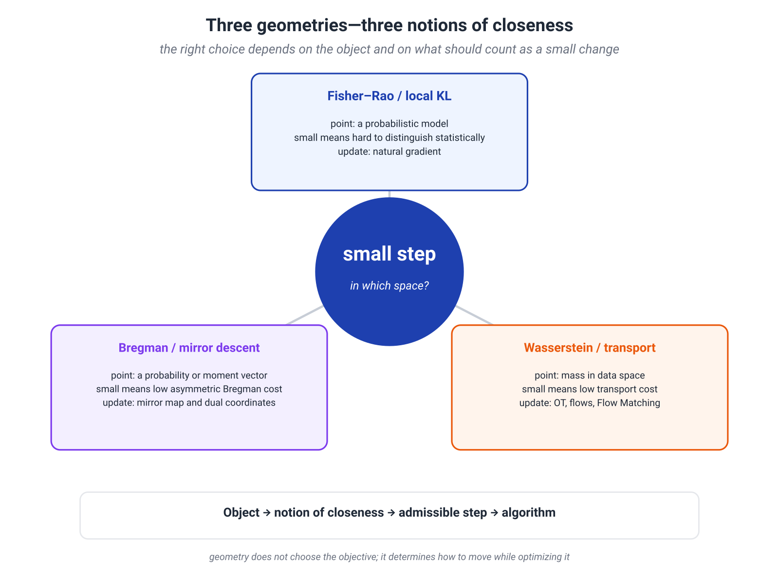
A useful compact statement is:
A geometry is a contract about which changes count as small.
For a policy, smallness may mean a small average KL between action distributions. For a model that transports noise into data, it may mean a small displacement in pixel or feature space. For ordinary deterministic regression, Fisher may not be the relevant object at all.
We begin with the geometry of neighboring distributions.
15.2. Fisher Information and the Local Form of KL
Let a model define a smooth family of distributions
The vector
is the parameter score function. Under standard regularity conditions its mean is zero:
The Fisher information matrix is
For any direction , its quadratic form has a transparent interpretation:
If this number is large, moving along noticeably changes the log probabilities of typical observations. Neighboring models are easier to distinguish in that direction. If the number is zero, a small move along does not change the represented distribution to first order.
Why Fisher Appears from KL
Consider a neighboring model . Expand its log density around :
Insert this expansion into
The linear term vanishes because the score has zero mean. When differentiation can be exchanged with integration,
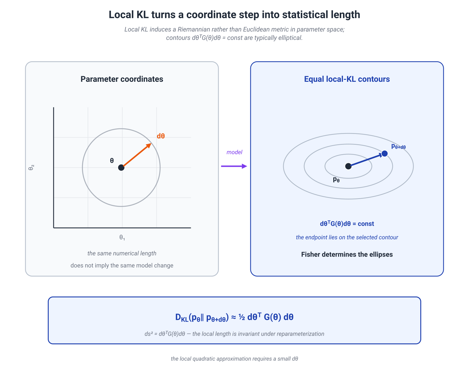
Hence
Read this formula in words:
Fisher information is the second-order cost of a small distributional change measured by KL.
Forward and reverse KL share the same quadratic term. Their asymmetry appears at higher orders. Fisher therefore defines a local Riemannian geometry, but it does not turn KL itself into a global metric: KL remains asymmetric and does not satisfy the triangle inequality.
Why the Length Is Coordinate Independent
Suppose the same model is written in new coordinates , with and
Then
while
Therefore
The entries of the matrix change, but the local statistical length does not. This is what it means for Fisher to transform as a metric tensor rather than as an arbitrary preconditioner.
An Exact Example: Bernoulli
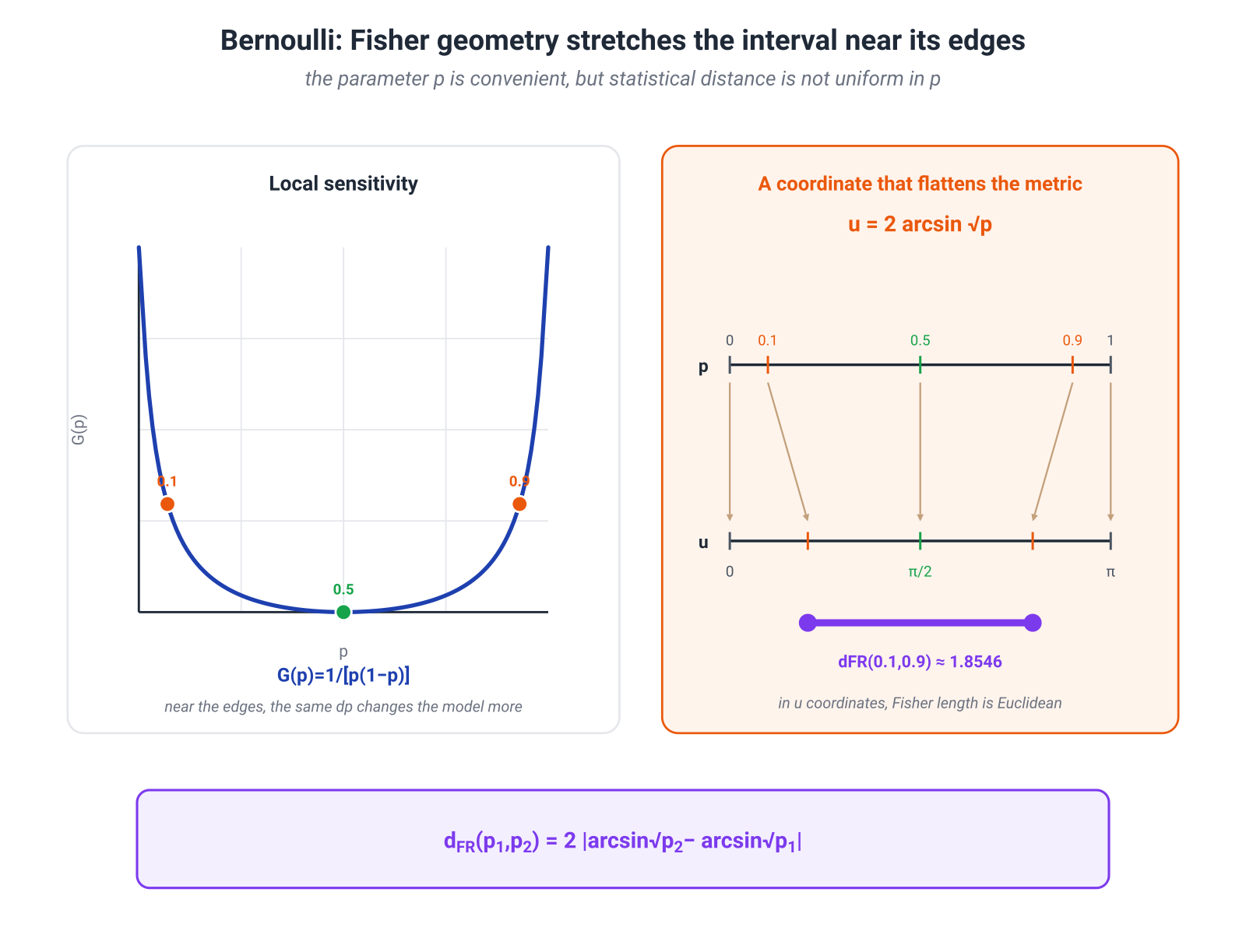
For in the coordinate,
In logit coordinates,
The two expressions look opposite: one diverges near the edge of the simplex, while the other tends to zero. Yet the line element is the same:
The coordinate
straightens this one-dimensional geometry:
Thus the exact Fisher–Rao distance between two Bernoulli distributions is
For and ,
The Same Matrix Limits Estimation Accuracy
For independent observations and an unbiased estimator under the usual regularity assumptions, the Cramér–Rao bound gives
This is another side of the same idea. If neighboring distributions are easy to distinguish, the parameter can be estimated more precisely. If different parameter values barely alter the observation law, no unbiased estimator can recover high precision from the same data.
Where the Local Picture Ends
Three boundaries matter.
- The quadratic approximation is reliable only for sufficiently small steps.
- Positive definiteness requires local identifiability. Symmetries and redundant parameters often make Fisher singular in deep networks.
- Fisher depends on which observation distribution and conditional model were declared to be the statistical object. “The Fisher matrix of the network” is incomplete until the expectations are specified.
The last point will become central in §15.4. First we derive the update induced by measuring step size with Fisher.
15.3. Natural Gradient: Steepest Descent Under Small Model Change
Suppose we minimize and write
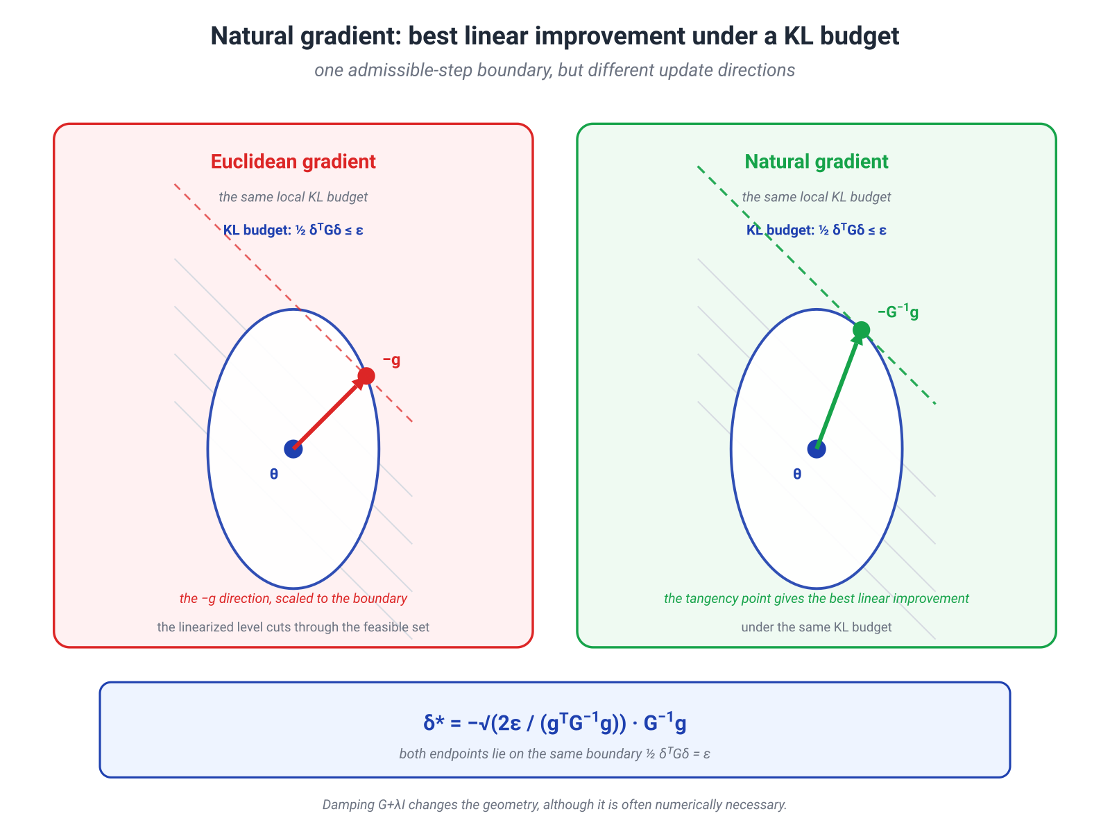
The ordinary gradient is the steepest descent direction under an Euclidean constraint. If smallness is measured by local KL, the optimization problem becomes
The Lagrangian gives the direction
where is an inverse or pseudoinverse. If is nonsingular, the step that uses the full budget is
Consider
The Euclidean gradient moves equally in both coordinates. The natural-gradient direction is
The first coordinate is one hundred times more sensitive in distribution space, so the same statistical budget permits a much smaller displacement there.
Coordinate Invariance in the Bernoulli Example
Let the objective depend on the probability: . In the coordinate, the natural-gradient flow is
In logit coordinates,
so
Transforming back,
Both coordinate systems describe the same continuous flow of distributions. Ordinary gradient flow does not have this property.
This is the strong positive result of natural gradient: the vector field transforms correctly under a smooth one-to-one reparameterization of the statistical model.
Why a Finite Step Still Depends on the Implementation
A practical algorithm does not take an infinitesimal displacement. It takes an Euler step:
After a nonlinear coordinate change, the finite endpoints agree only to first order in . Exact finite-step invariance would require geodesic integration or a compatible retraction.
Practical implementations therefore rely on
- small or adaptively chosen steps;
- checking the realized KL after the update;
- line search;
- damping;
- and an adequate approximation to the curvature matrix.
The damped step
is often numerically essential. Yet the added introduces an Euclidean component and therefore changes the original geometry. It is a useful engineering compromise, not a neutral detail.
Natural Gradient Is Not Newton’s Method
Newton’s method uses the Hessian of the objective:
Natural gradient uses the Fisher matrix of the statistical model:
They can coincide in special likelihood settings—for example at the level of an expected negative log likelihood under appropriate model specification. In neural networks, Fisher is also closely related to the generalized Gauss–Newton matrix for several exponential-family output distributions. But the empirical Hessian, model Fisher, and GGN differ in general. Martens gives a detailed account of these relationships and their optimization consequences. (Martens, 2020)
A useful summary is:
The inverse Fisher is not a magical accelerator. It changes the units of the step so that equal budgets correspond approximately to equal changes in the model distribution.
15.4. What “Curvature” Is Actually Used in a Deep Network?
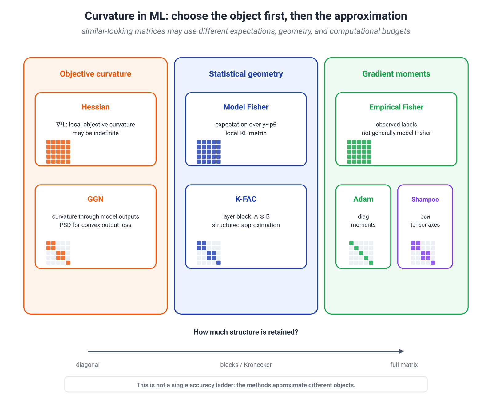
The full Fisher matrix of a model with billions of parameters cannot be stored or inverted directly. Before discussing approximations, however, we must decide which matrix is being approximated.
Model Fisher
For a conditional model and an input distribution ,
where
The crucial detail is that the inner expectation samples labels from the current model.
Empirical Fisher
On a dataset one often computes
Here the labels come from the data, not from . This matrix is the second moment of observed per-example gradients, but in general it is not an unbiased estimator of the model Fisher and need not approximate the Hessian. Kunstner, Balles, and Hennig analyze this distinction and its pathologies in detail. (Kunstner et al., 2019)
A small example shows the size of the mismatch. For a Bernoulli model in logit coordinates,
If the data have true positive rate , the population second moment of the observed gradient is
At
we obtain
Both quantities are built from squared gradients, but they answer different questions.
Generalized Gauss–Newton
Let the network output be and the loss be . The generalized Gauss–Newton matrix is
where is the Jacobian of the output with respect to parameters and is the Hessian of the loss with respect to the output. If is convex in , GGN is positive semidefinite. For some probabilistic output models it coincides with the appropriate Fisher matrix, but this requires a specific output parameterization and loss.
K-FAC, Adam, and Shampoo
K-FAC approximates large Fisher or GGN blocks by Kronecker products:
The factor describes input-activation statistics, while describes backpropagated-gradient statistics. This makes an approximate inverse much cheaper to apply, but only part of the correlation structure is retained and damping remains necessary. K-FAC was introduced explicitly as an efficient approximation to natural gradient descent. (Martens & Grosse, 2015)
Adam tracks coordinatewise first and second moments of stochastic gradients and scales updates by roughly
This is an adaptive diagonal preconditioner. Squared gradients may resemble a diagonal empirical-Fisher statistic, but Adam does not invert the model Fisher and does not inherit full natural-gradient invariance.
Shampoo constructs structured second-moment matrices along tensor axes. It is related to full-matrix AdaGrad and preserves more structure than coordinatewise methods, but it is not automatically a Fisher approximation.
| Method | Object used | Structure retained | What it does not guarantee automatically |
|---|---|---|---|
| Newton | objective Hessian | local curvature of the objective | statistical reparameterization invariance |
| Natural gradient | model Fisher | local KL geometry | an exact global trust region |
| GGN | output-loss curvature | positive semidefiniteness for convex output losses | equality with Fisher in every task |
| Empirical Fisher | second moment of observed gradients | direct availability from data | correct Fisher geometry away from special regimes |
| Adam | coordinatewise gradient moments | cheap adaptive scaling | natural-gradient invariance |
| K-FAC | Kronecker blocks of Fisher/GGN | within-layer cross-coordinate structure | exact inversion of the full matrix |
| Shampoo | tensor-structured second moments | structure across parameter axes | a Fisher interpretation without extra assumptions |
That is the practical lesson: the word “curvature” does not identify one universal matrix. Each method decides which dependencies to retain, which to discard, and how much computation to spend on them.
15.5. Policy Geometry: NPG, TRPO, PPO, and KL in RLHF
A policy is itself a conditional distribution:
The idea of measuring a small distributional change is therefore especially natural. For a chosen state distribution , the policy Fisher matrix is
The natural policy gradient is
It rescales the update so that sensitive directions in the action distribution move more cautiously.
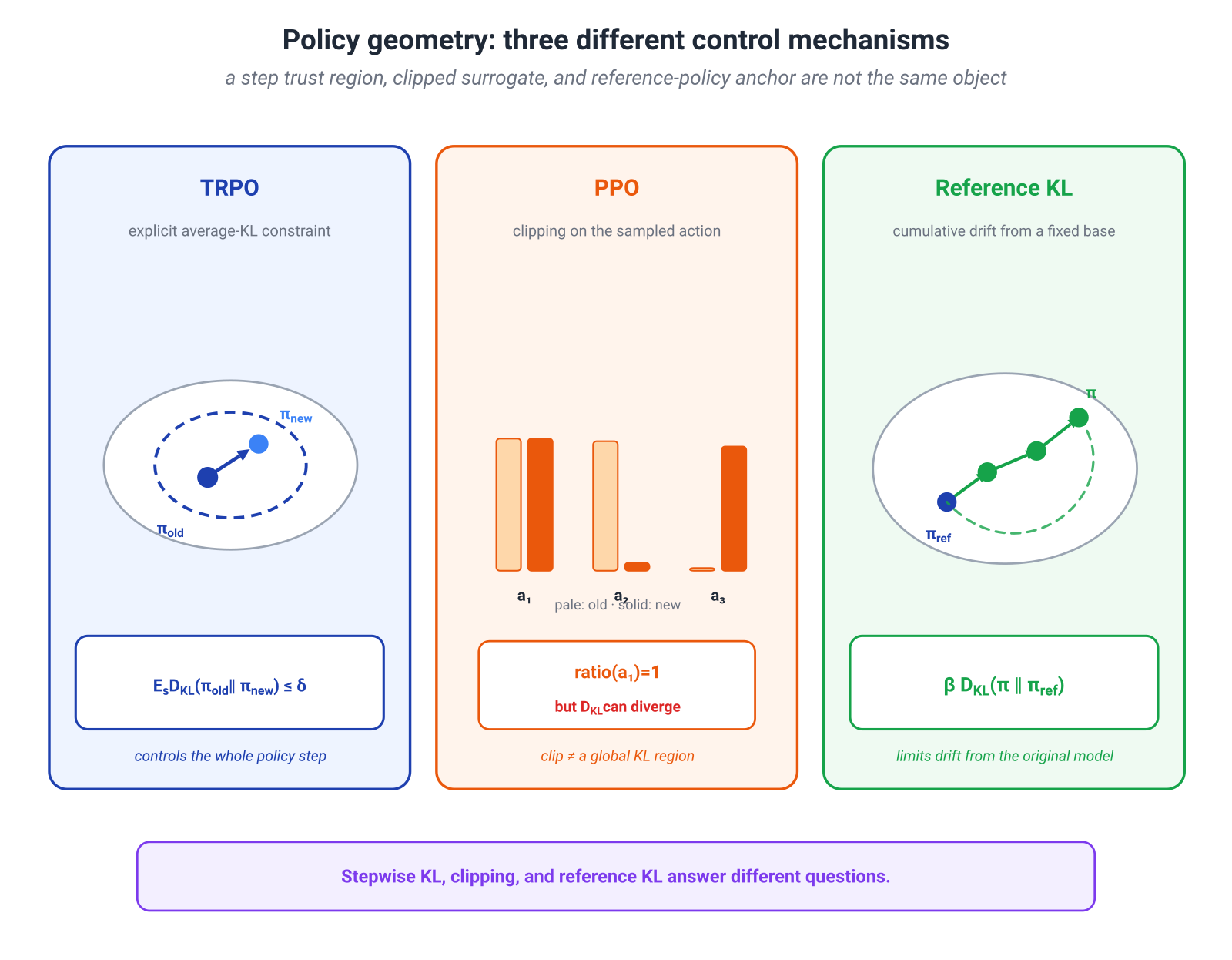
TRPO: A Trust Region in Policy Space
TRPO starts from a local surrogate objective and constrains the average policy change:
Linearizing the objective and quadratically approximating the KL yields the same constrained problem as in §15.3, hence a natural-gradient direction. Practical TRPO uses conjugate gradients and line search rather than an exact geodesic. The original paper explicitly derives the practical method through a sequence of approximations to a theoretically motivated trust-region update. (Schulman et al., 2015)
Two levels should be kept separate:
- theoretical improvement bounds use stronger control of distribution shift;
- the practical algorithm controls an empirical average KL and checks the step numerically.
PPO: A Useful Proxy, Not a Hard Trust Region
PPO uses the probability ratio
and the clipped surrogate
This supports multiple epochs of minibatch updates and often stabilizes optimization. Yet clipping controls ratios for actions observed in the sample, not the entire policy.
A three-action counterexample makes this explicit. Let
and suppose the batch contains only the first action. Consider
The sampled-action ratio is always one, so the corresponding sampled surrogate is unchanged. But
as . Thus clipping is not a global KL constraint. Implementations commonly monitor approximate KL, stop early, or add an explicit penalty. PPO was proposed as a simpler first-order method with some practical benefits of TRPO, not as an exact solution to the same constrained problem. (Schulman et al., 2017)
Two Different KL Terms in RLHF
RLHF-style training can contain two distinct constraints.
- Stepwise KL compares the current policy with the snapshot that generated the data for the present update. It limits the size of one optimization step.
- Fixed-reference KL compares the current model with a fixed SFT or reference model. It limits accumulated drift over the whole run.
A compact way to remember the distinction is:
TRPO asks, “How far did we move this step?” Reference KL asks, “How far have we drifted from the starting model?”
For a fixed context, the idealized problem
has the exact Gibbs optimum
Module 8 gave the full derivation. Here the geometric reading matters: KL prices departure from the reference distribution, and the exponential tilt is the exact proximal solution of the idealized objective.
DPO uses this analytic relation to express preferences through policy-to-reference log ratios. It does not perform a natural-gradient or TRPO step on every minibatch. Shared KL algebra does not make the algorithms identical.
One more boundary: policy KL in RLHF compares response distributions, whereas PAC-Bayes KL in Module 12 compares distributions over hypotheses. The same formula does not transfer a generalization certificate from one setting to the other.
15.6. Wasserstein Geometry and Distribution Flows
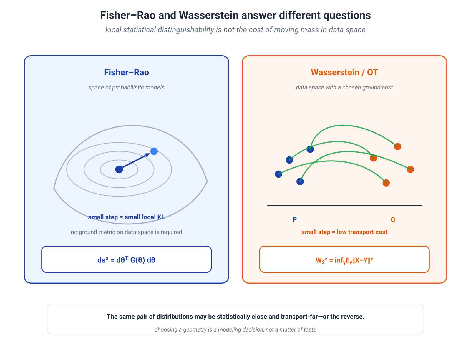
Fisher geometry answers how distinguishable neighboring models are. Sometimes, however, the crucial structure lies in the observation space itself.
Consider two point masses:
For every , the supports are disjoint. Both directed KL divergences are infinite, total variation is one, and Jensen–Shannon is , whether the second point is or units away.
Wasserstein sees the relevant structure:
It uses the geometry of the data space.
Definition Through a Transport Plan
With quadratic cost,
A coupling specifies which mass from is paired with which mass from . The ground metric is part of the problem. Rescaling one coordinate changes the transport cost.
Dynamic Form
The Benamou–Brenier formula expresses the same distance as minimal kinetic action:
subject to the continuity equation
The point in the space is now a full distribution , and the vector field transports its mass. Not every path between and is a geodesic; a geodesic minimizes the action.
Continuous Normalizing Flows
Let a particle follow the ODE
Then its density evolves along the trajectory according to
This is the continuous counterpart of the change-of-variables formula and underlies continuous normalizing flows. Neural ODEs showed how to train such models and compute likelihoods through the integrated divergence. (Chen et al., 2018)
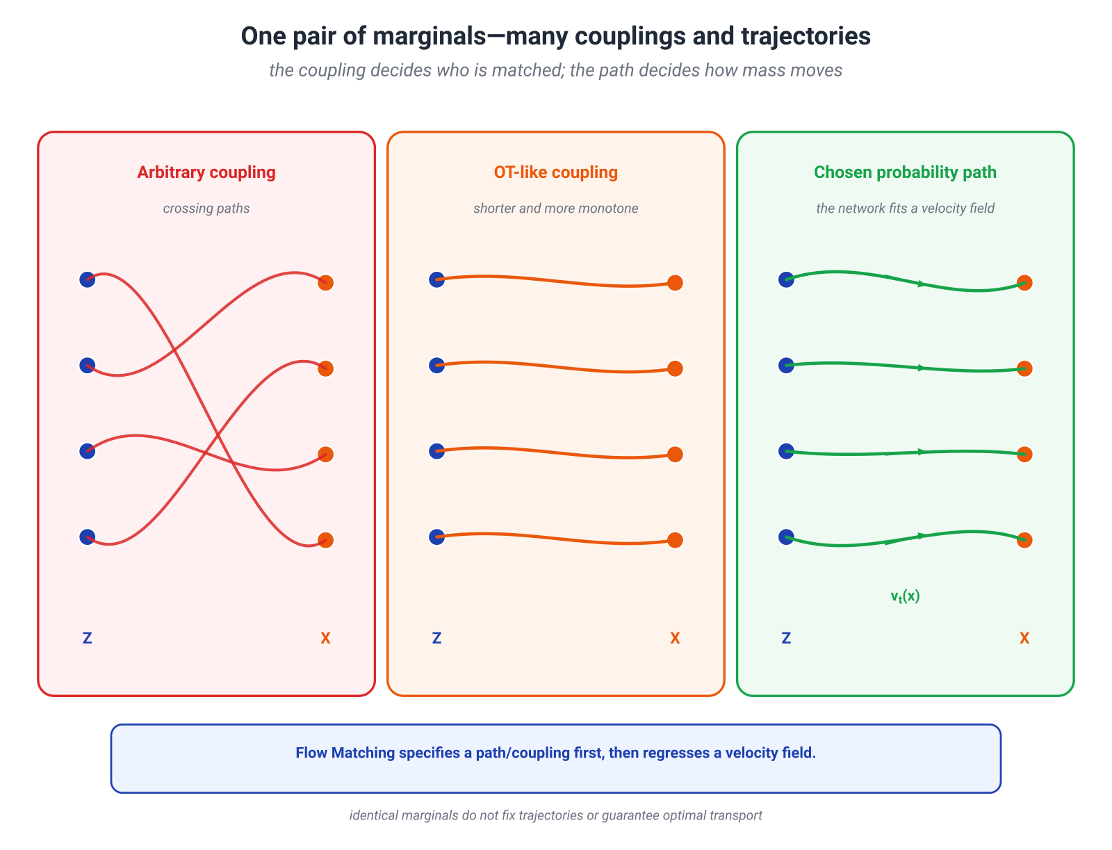
Flow Matching: The Path Is Chosen First
Flow Matching does not begin by evaluating an unavailable log density. One chooses a family of intermediate distributions or conditional probability paths and trains a neural vector field by regression to the velocity that realizes the chosen evolution.
There are two central design freedoms:
- the coupling between initial and final points;
- the path used between each coupled pair.
The same endpoint marginals permit many couplings, and therefore many velocity fields and trajectories. Flow Matching is compatible with diffusion paths as well as paths based on optimal-transport displacement interpolation. This flexibility is part of the original method. (Lipman et al., 2022)
In one-dimensional Gaussian transport the role of the coupling is especially clear. Let
share the same . The interpolation
is the Wasserstein geodesic between the Gaussian marginals. If and are sampled independently, the endpoints remain correct but the kinetic action is larger. A coupling is not bookkeeping; it determines the path geometry.
Rectified Flow
Rectified Flow trains an ODE to follow straight lines between pairs drawn from a chosen coupling and may repeatedly “rectify” the resulting transport. The original work shows that rectification does not increase convex transport costs of the induced coupling and can produce trajectories that are easier to simulate with coarse discretization. (Liu, Gong & Liu, 2022)
This does not imply that every trained rectified flow is the exact optimal-transport map or a global Wasserstein geodesic. Path straightness, coupling quality, regression error, and numerical integration error are distinct issues.
Probability-Flow ODE and Diffusion
For the SDE
with scalar state-independent diffusion coefficient, the corresponding probability-flow ODE has drift
With the exact score, the SDE and ODE have the same one-time marginals . Their trajectories and couplings differ: one is stochastic and the other deterministic. This equivalent neural ODE is derived in the score-based SDE framework. (Song et al., 2021)
Finally, distinguish two scores:
is a gradient in observation space used in diffusion, whereas
is a parameter-space natural gradient transformed by Fisher geometry. Both involve distributions and gradients, but they live in different spaces.
15.7. Exponential Families, Dual Coordinates, and Mirror Descent
Module 8 derived the exponential-family form
We can now read it geometrically.
The expectation parameters are
and the Fisher matrix is
KL between two family members is a Bregman divergence of the log-partition function:
The order matters: the tangent to is taken at and evaluated at . In dual coordinates,
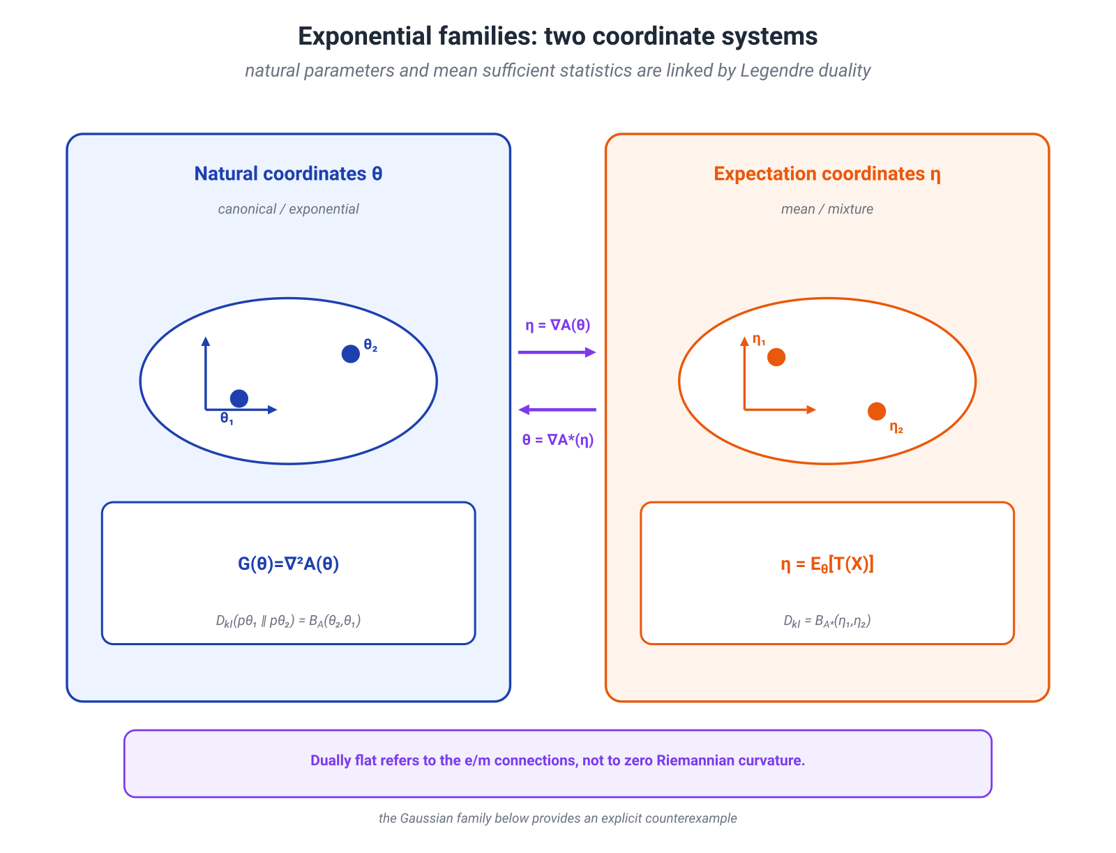
Natural coordinates and expectation coordinates form two affine coordinate systems related by Legendre duality. This is the meaning of a dually flat structure. “Flat” refers to the pair of e/m affine connections; it does not imply zero Riemannian curvature for the Fisher–Rao Levi–Civita connection. The Gaussian family in §15.9 gives an explicit counterexample.
Mirror Descent
A mirror-descent step has the form
where is the Bregman divergence generated by a convex function .
On the probability simplex, the natural choice
gives
The update is
This is the same exponential tilt that appeared in Module 8. There it arose as a MaxEnt or KL-regularized optimum; here it appears as a proximal update on the simplex.
Locally, a Bregman divergence has the quadratic form
Mirror descent and natural gradient are therefore closely related through the corresponding local metric; in exponential families the relation is especially clean in dual coordinates. Globally they are not the same algorithm for an arbitrary and a finite step. Mirror descent uses the full asymmetric Bregman divergence, while natural gradient uses its local quadratic metric. Raskutti and Mukherjee analyze this equivalence on the dual Riemannian manifold of exponential families. (Raskutti & Mukherjee, 2013)
15.8. Practical Map: Choose the Object Before the Geometry
After all these formulas, one final overreach is tempting: call Fisher “the true geometry of machine learning,” or replace it everywhere with Wasserstein. The useful map is more modest.
| Task | Point in the space | Meaning of a small change | Useful construction |
|---|---|---|---|
| likelihood model | neighboring distributions are hard to distinguish | Fisher / local KL | |
| policy update | action distributions change little on relevant states | state-averaged policy KL / Fisher | |
| simplex weights | distribution | small Bregman cost from the current point | mirror descent / KL |
| sample transport | distribution in data space | mass moves a short distance | Wasserstein / OT |
| deterministic regression | parameters or outputs | small task-specific functional error | Hessian, GGN, or a task metric |
| large network | structured parameter blocks | a useful curvature is approximated within budget | K-FAC, Shampoo, adaptive preconditioners |
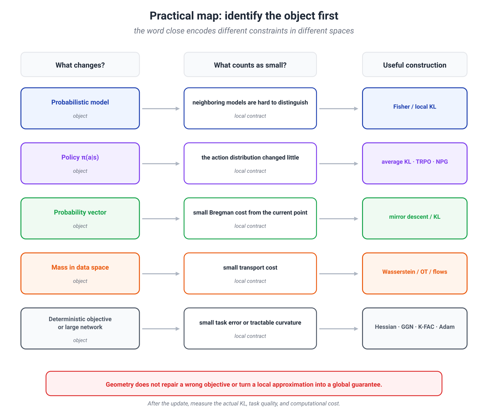
Before using geometric language, ask five questions.
- What is the object being updated? Parameters, response distributions, representations, or sample paths?
- What should count as small? KL, transport cost, logit change, or task error?
- Is the approximation local? If so, is the realized step actually small enough?
- Which matrix or divergence does the code compute? Model Fisher, empirical Fisher, GGN, or only a diagonal moment?
- What is checked after the update? Realized KL, task quality, integration cost, or policy drift?
The central synthesis is:
Geometry does not choose the learning objective. It determines which motions count as nearby while optimizing that objective.
Natural gradient cannot repair a misspecified reward. Wasserstein does not guarantee a convenient path for a finite neural network. K-FAC does not make a nonconvex problem convex. But an appropriate geometry can remove artificial coordinate dependence, make a trust region meaningful, and identify which curvature structure is worth preserving.
15.9. Mathematical Deepening: α-Geometry and Exact Examples
Optional on a first pass. The main ML route is complete. Here we examine how one Fisher metric can coexist with several asymmetric connections, and we write two geodesies in closed form.
α-Divergences in Amari’s Convention
For ,
The limits are
At one obtains a constant multiple of squared Hellinger distance.
This is Amari’s geometry parameter, not the order of Rényi divergence. Different sign and scaling conventions exist, so the limits must be read together with the definition.
All smooth α-divergences in this family induce the same Fisher metric at second order. Their difference appears at third order and determines different affine connections:
- : e-connection;
- : m-connection;
- : the Fisher-metric Levi–Civita connection.
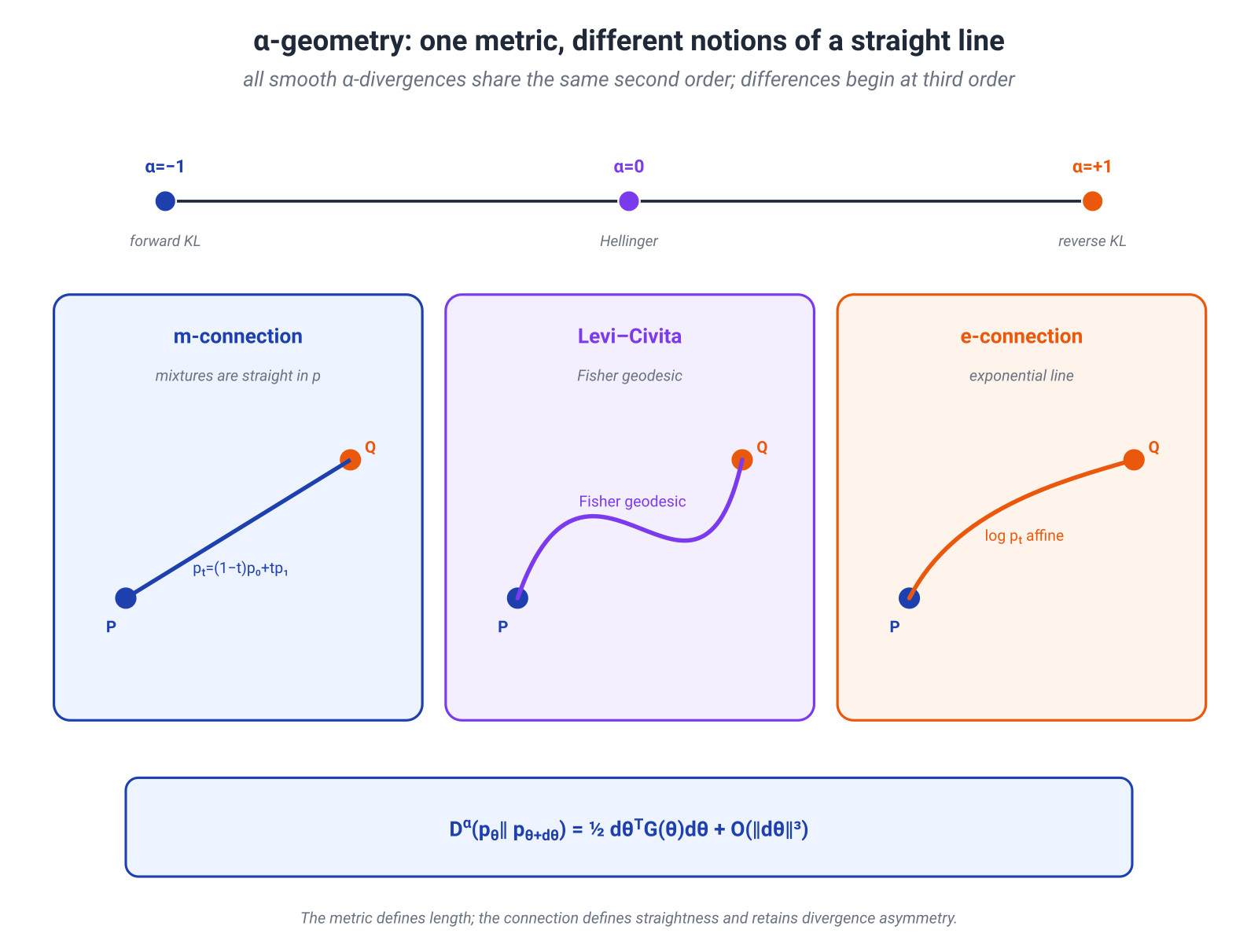
This is the key conceptual point: a metric describes local length, but a metric alone does not recover the asymmetry of a divergence or its notion of a straight line.
Categorical Distributions as Part of a Sphere
For an interior categorical distribution , the Fisher line element is
Set
Then
and
Thus the interior of the simplex maps to the positive orthant of a sphere of radius . The exact distance is
For this reduces to the Bernoulli formula from §15.2. The coefficient
already appeared in Module 11 as the Bhattacharyya coefficient and in Hellinger distance. Here it becomes the cosine of a spherical angle.
Bernoulli Geodesic
In the coordinate
the geodesic is an ordinary line:
Transforming back,
It is not the linear probability interpolation .
The Normal Family and the Hyperbolic Plane
For
Fisher in coordinates is
Let
Then
This is a scaled Poincaré upper-half-plane metric with constant Gaussian curvature
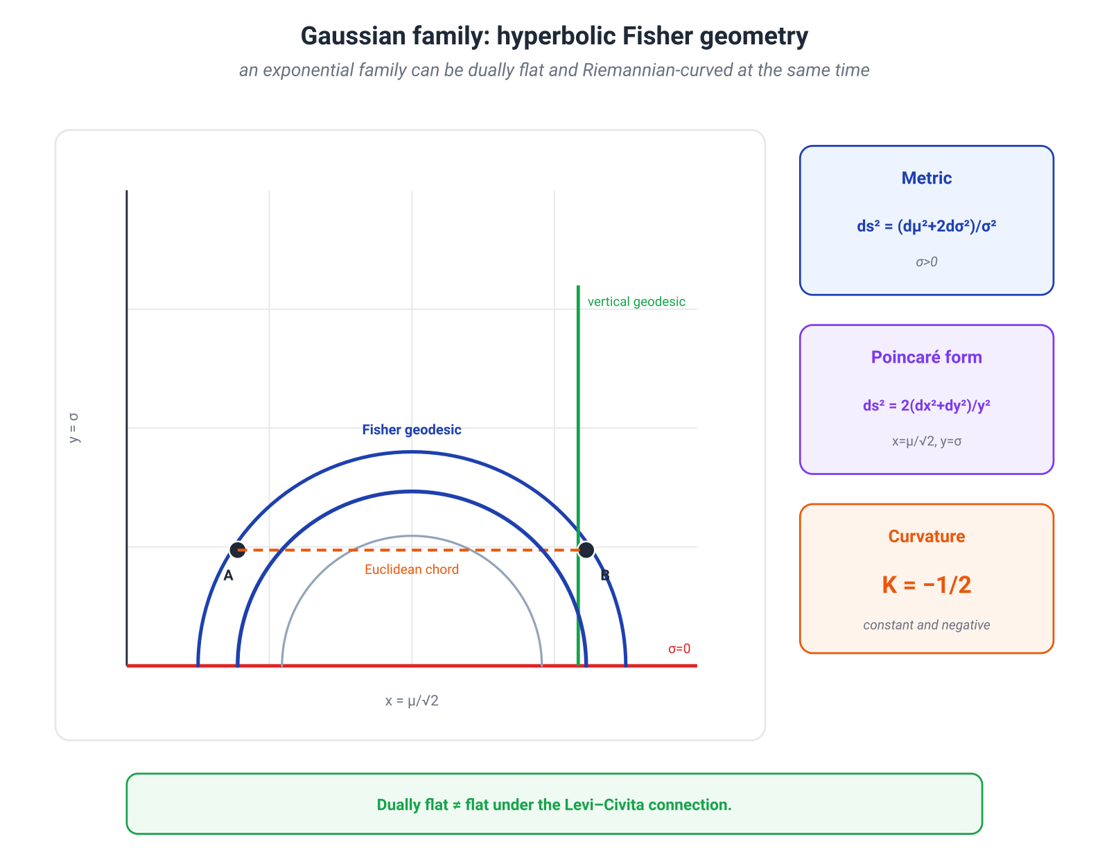
Thus the normal family is an exponential family and is dually flat, but it is not Riemann-flat with respect to the Fisher–Rao Levi–Civita connection. The two uses of “flat” refer to different connections.
Chentsov’s Theorem
In classical finite-dimensional statistics, Chentsov’s theorem says, roughly, that up to an overall scale the Fisher–Rao metric is the unique Riemannian metric on probability simplices compatible with sufficient statistics and suitable stochastic mappings.
This is a powerful justification for Fisher as a statistical geometry. It does not imply that Fisher is the correct cost for moving images, physical coordinates, or hidden states. The ground metric of the data space does not appear in the theorem. Wasserstein answers a different question, so the two constructions do not compete.
15.11. Conclusion
By the end of the course, familiar information quantities have acquired another role. Entropy and KL began as bills for uncertainty and model mismatch. Their second-order behavior now defines the local shape of distribution space and changes what a gradient step means.
Three questions keep the map clear:
- Fisher–Rao: how distinguishable are neighboring probabilistic models?
- Bregman geometry and mirror descent: how should a constrained distribution be updated relative to its current point?
- Wasserstein: what does it cost to physically move probability mass through data space?
These geometries cannot be substituted for one another mechanically. Together, however, they organize a broad range of modern ML methods:
The main lesson is not that every popular algorithm is “really” one geometric theorem. It is this:
First define the object, then define what closeness means, and only then choose a geometry and a computable approximation to it.
Information geometry closes the course not with one more universal slogan, but with a discipline of problem formulation. A formula becomes stronger when we know exactly what it measures—and where its promise ends.
Main Sources
- S.-I. Amari, Information Geometry and Its Applications, Springer, 2016.
- S.-I. Amari, Natural Gradient Works Efficiently in Learning, 1998.
- J. Martens, New Insights and Perspectives on the Natural Gradient Method, 2020.
- J. Martens and R. Grosse, Optimizing Neural Networks with Kronecker-factored Approximate Curvature, 2015.
- F. Kunstner, L. Balles, and P. Hennig, Limitations of the Empirical Fisher Approximation, 2019.
- S. Kakade, A Natural Policy Gradient, NeurIPS 2001.
- J. Schulman et al., Trust Region Policy Optimization, 2015.
- J. Schulman et al., Proximal Policy Optimization Algorithms, 2017.
- R. Rafailov et al., Direct Preference Optimization, 2023.
- R. T. Q. Chen et al., Neural Ordinary Differential Equations, 2018.
- Y. Lipman et al., Flow Matching for Generative Modeling, 2022.
- X. Liu, C. Gong, and Q. Liu, Flow Straight and Fast, 2022.
- Y. Song et al., Score-Based Generative Modeling through Stochastic Differential Equations, 2021.
- G. Raskutti and S. Mukherjee, The Information Geometry of Mirror Descent, 2013.