Module 9. Rate–distortion and the Information Bottleneck: managing information loss

How to read this module. Sections 9.1–9.8 form the main route. We begin with classical rate–distortion theory, then move to the Information Bottleneck, its variational form, VAEs, and practical compression and quantization. Section 9.9 is a mathematical extension on I–MMSE and Gaussian noising; it can be saved for a second pass. Section 9.10 contains the exercises.

9.1. Why a model may need to forget

Module 6 can leave us with a correct but incomplete intuition: preserving more information is always better. For lossless compression, that is exactly the contract—the decoder must recover the source object perfectly.

Most ML systems solve a different problem.

An image of a handwritten digit contains the digit class, the writer's identity, stroke width, position on the canvas, background texture, and sensor noise. A digit classifier can discard some of these differences. A writer-identification system cannot. Exact reconstruction needs still more detail.

The same information may be:

• useful signal for one task;
• nuisance variation for another;
• an indispensable part of the source for a third.

The word “irrelevant” therefore has no meaning without a task.

JPEG may discard fine high-frequency detail to produce a smaller file. A neural codec may spend more bits on a face than on a smooth background. A classifier encoder may suppress illumination while preserving shape. An LLM quantizer may round many weights aggressively as long as the predictive distribution changes little.

All of these systems face the same question:

What is the minimum amount of information that must be retained to keep performance acceptable under a chosen criterion?

A bottleneck is not an instruction to forget as much as possible. It is a contract: what may be lost, at what cost, and for which task.

This module connects four constructions:

1. rate–distortion theory asks how many bits are needed at a permitted level of loss;
2. the Information Bottleneck (IB) derives the cost of forgetting from a variable we want to predict;
3. the Variational Information Bottleneck (VIB) and VAE replace inaccessible information quantities with trainable variational objectives;
4. learned compression and quantization show when an abstract “rate” becomes an actual number of bits and when it remains a useful surrogate.

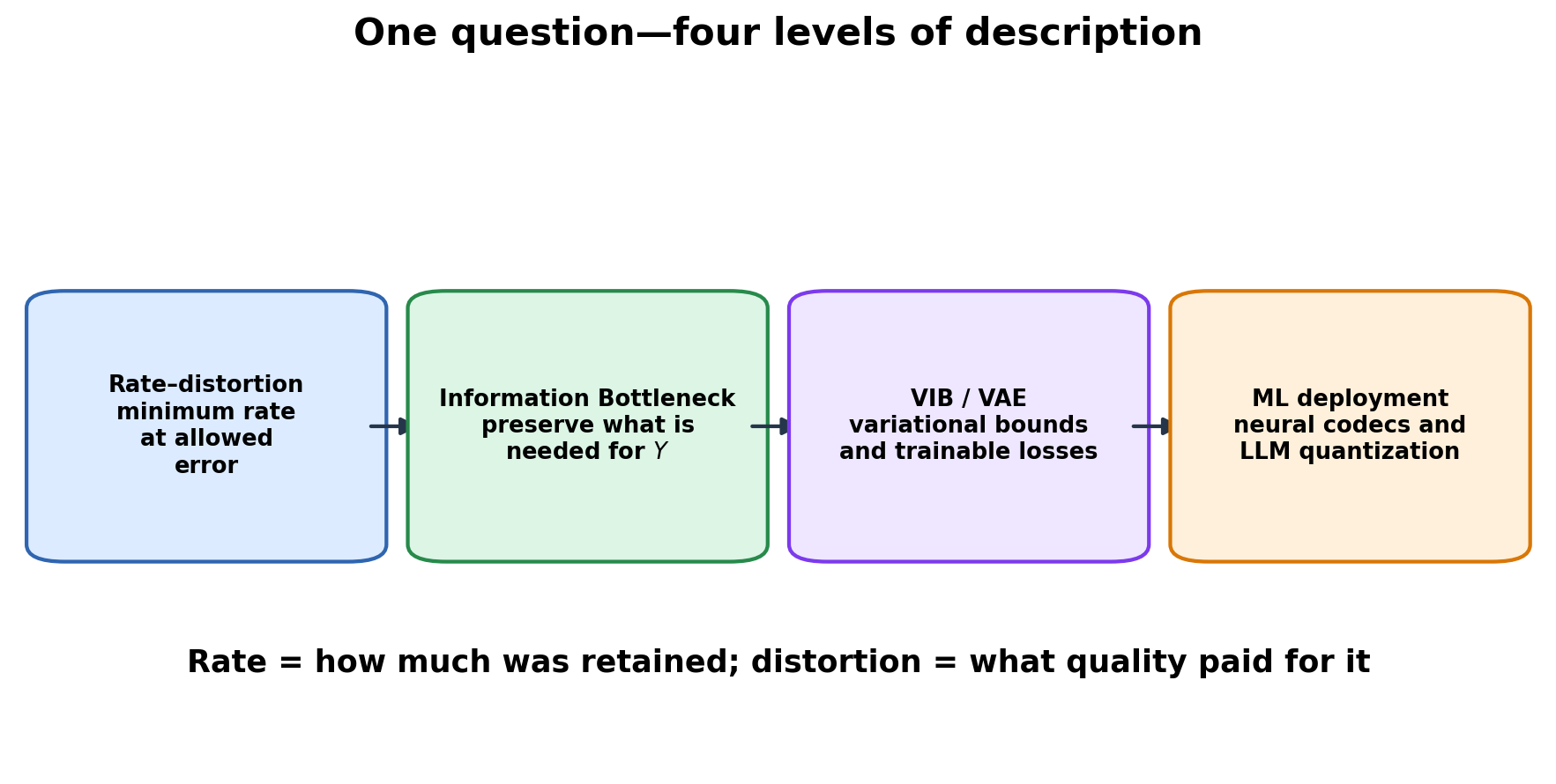
The recurring pair of concepts is:

• rate—how much information passes through the representation;
• distortion—what quality is sacrificed to reduce that rate.

Unless stated otherwise, classical rate–distortion formulas use bits. Variational ML objectives are usually implemented with natural logarithms and measured in nats. We will state the logarithm base whenever it changes a numerical coefficient.

9.2. Rate–distortion theory: how much information must be retained

From two extreme codes to an entire curve

Let

$$X\sim\operatorname{Bernoulli}(0.25),$$

with Hamming distortion

$$d(x,\widehat x)=\mathbf 1\{x\ne\widehat x\}.$$

Two solutions are immediate.

Exact coding. Perfect recovery asymptotically requires

$$H_2(X)=h_2(0.25)\approx0.811\ \text{bits per symbol}.$$

Zero rate. Send nothing and always reconstruct $\widehat X=0$. The rate is zero and the average distortion is

$$P(X=1)=0.25.$$

An entire family of compromises lies between these points. If we allow average distortion $D=0.1$, the optimal asymptotic rate is already

$$R(0.1)=h_2(0.25)-h_2(0.1)\approx0.342\ \text{bits per symbol}.$$

Rate–distortion theory describes this boundary: how much information is unavoidably required at each permitted reconstruction quality.

Formal setup

Let a source produce $X\sim P_X$, and let the decoder construct a reproduction $\widehat X$ in a reproduction alphabet $\widehat{\mathcal X}$. A distortion function

$$d(x,\widehat x)\ge0$$

assigns a cost to replacing $x$ by $\widehat x$.

Common choices include:

• Hamming distortion: $\mathbf 1\{x\ne\widehat x\}$;
• squared error: $(x-\widehat x)^2$;
• negative log-likelihood under a reconstruction model;
• KL divergence between the outputs of the original and compressed models;
• a perceptual distance in feature space;
• degradation on a downstream task.

For a discrete memoryless source, the rate–distortion function is

$$\boxed{ R(D) = \inf_{P_{\widehat X\mid X}:\ \mathbb E[d(X,\widehat X)]\le D} I(X;\widehat X) }.$$

The conditional distribution $P_{\widehat X\mid X}$ is called a test channel. It need not be a physical communication channel or a finished coding algorithm. It specifies the desired joint law of source symbols and reproductions: which substitutions are allowed and how often they occur.

Why mutual information becomes a bit rate

At first sight, the definition contains neither files nor codewords—only mutual information. Its operational meaning appears over long blocks.

Under the standard assumptions, Shannon's theorem states that:

• every rate above $R(D)$ is asymptotically achievable at average distortion no larger than $D$;
• every rate below $R(D)$ is asymptotically insufficient.

The encoder does not have to describe each source symbol independently. It codes a long typical block and exploits the repeated statistical structure of the source. Once optimized over the test channel, mutual information becomes the minimum number of bits per source symbol.

This is the same intellectual move as in lossless source coding: local probabilities become the global geometry of long sequences.

The geometry of the trade-off

The function $R(D)$ is non-increasing and convex. Allowing more distortion cannot raise the minimum required rate. Convexity says that time-sharing between two coding regimes performs no worse than the corresponding average trade-off.

Zero rate is reached at

$$D_{\max} = \min_{\widehat x} \mathbb E[d(X,\widehat x)],$$

because a decoder that receives no message can only emit a fixed reproduction.

The statement $R(0)=H(X)$ requires assumptions. It holds for a finite discrete source when zero distortion requires exact reproduction. For a continuous source with squared error, one generally has

$$R(D)\to\infty \qquad\text{as}\qquad D\downarrow0,$$

because an exact real number requires unbounded precision.

In practice, one often optimizes the Lagrangian

$$I(X;\widehat X)+\lambda\,\mathbb E[d(X,\widehat X)].$$

At a differentiable operating point,

$$\lambda=-R'(D).$$

Thus $\lambda$ is a local exchange rate: how much additional rate we are willing to pay for a reduction in distortion. The same geometry will reappear in IB, VAEs, and learned compression.

Two benchmark sources

For $X\sim\operatorname{Bernoulli}(p)$, $p\le1/2$, under Hamming distortion,

$$R(D) = \begin{cases} h_2(p)-h_2(D), & 0\le D\le p,\\ 0, & D\ge p. \end{cases}$$

For a Gaussian source

$$X\sim\mathcal N(0,\sigma^2)$$

under squared error, using base-2 logarithms,

$$\boxed{ R(D) = \begin{cases} \dfrac12\log_2\dfrac{\sigma^2}{D}, & 0<D<\sigma^2,\\ 0, & D\ge\sigma^2. \end{cases} }$$

In this particular model, halving the MSE costs another $0.5$ bit per real-valued source symbol.

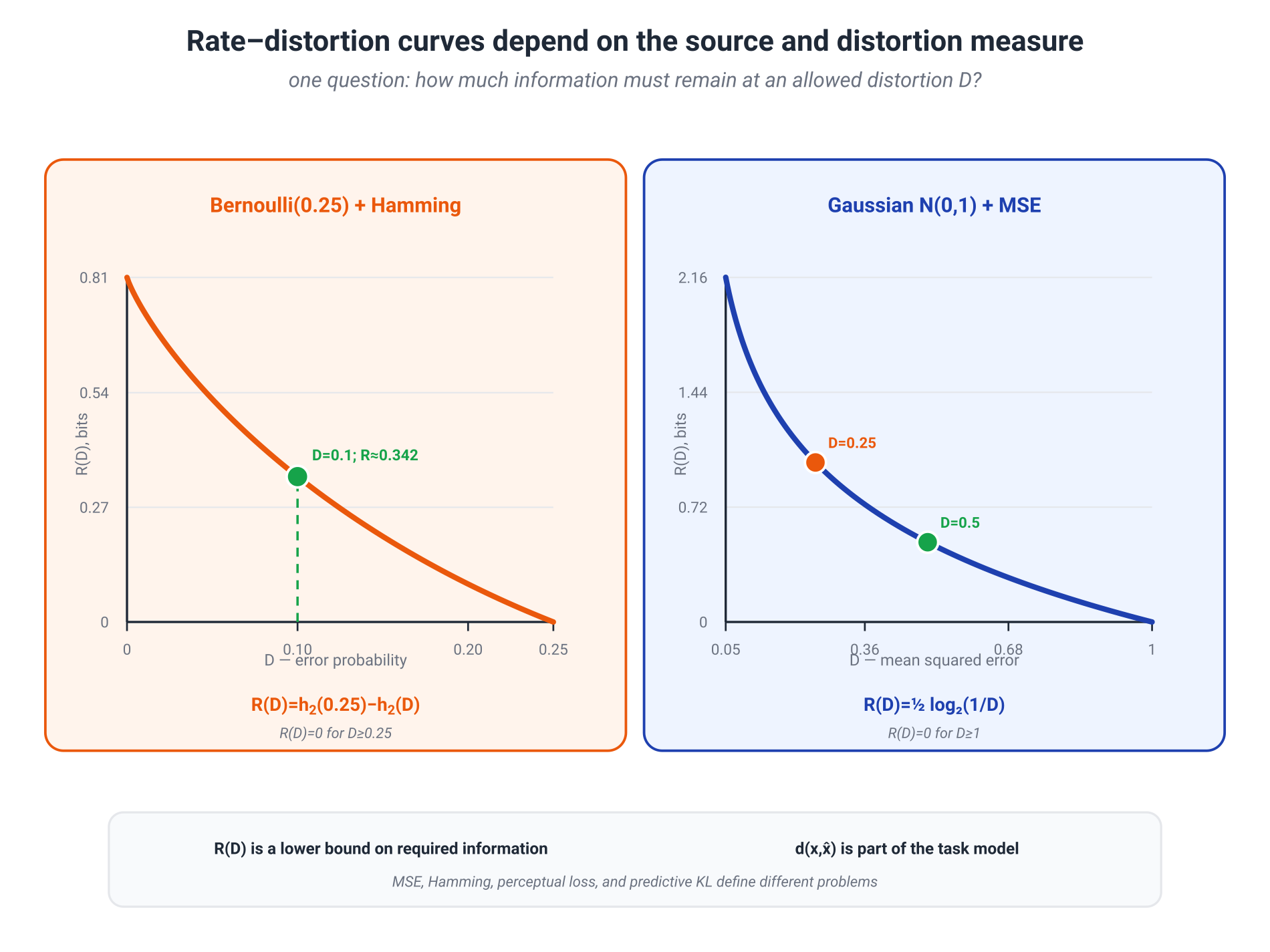
Distortion is not supplied by nature

This is where an overly broad conclusion is tempting. The theory finds the optimal code for a specified distortion function. It does not decide which errors matter to a person or a downstream system.

MSE aligns conveniently with a Gaussian likelihood and PSNR, but it may penalize a small image shift heavily and reward an averaged, blurry reconstruction. A perceptual loss may preserve visual structure better, but it inherits the assumptions of the selected feature network. For a compressed LLM, a natural distortion may be an increase in NLL or a KL divergence between predictive distributions rather than weight MSE.

Visual compression introduces a third object as well: the perceptual plausibility of the reconstruction distribution. Low expected distortion and realistic-looking samples are not identical goals; imposing an additional perception constraint generally raises the achievable rate–distortion boundary.

This does not weaken the theory. It forces us to name what engineering discussions often hide inside the word “quality.”

9.3. Information Bottleneck: preserve what matters for $Y$

Classical rate–distortion theory asks the engineer to provide $d(x,\widehat x)$. In representation learning, however, it is often unclear in advance which differences between inputs should matter.

Consider two images of the same digit. Their pixels, handwriting style, and background may differ. If their conditional label distributions are nearly identical, a classifier benefits from treating them as similar. If the target variable is writer identity, the same differences become relevant.

The Information Bottleneck lets the prediction task define the cost of forgetting.

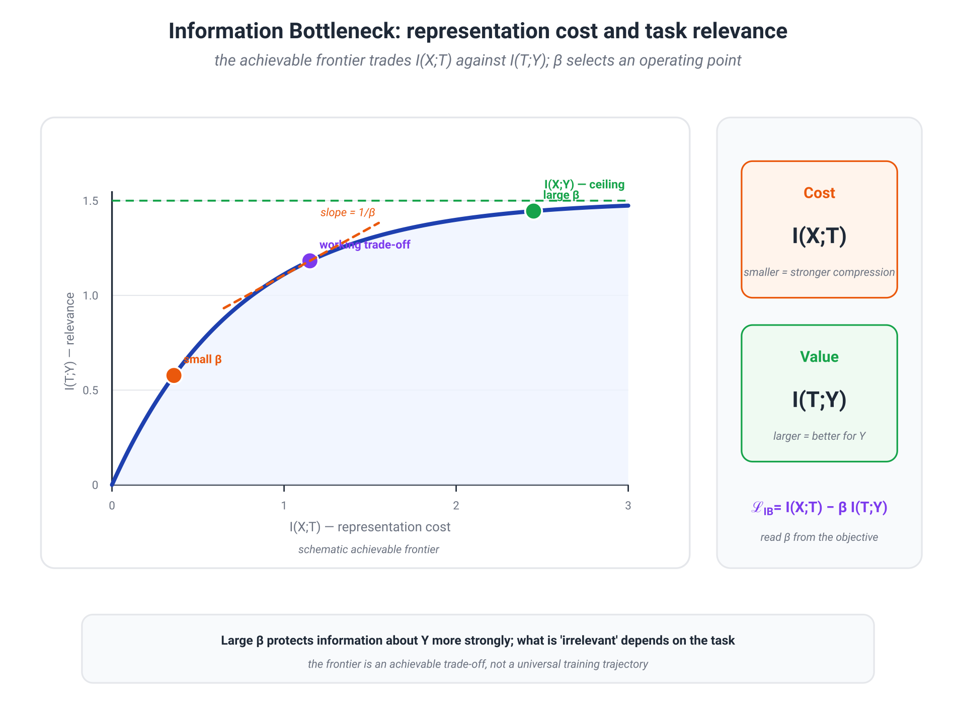
Let $Y$ be a relevant variable and let a representation $T$ be constructed only from $X$:

$$Y\longrightarrow X\longrightarrow T.$$

We want to:

• reduce $I(X;T)$, so the representation does not carry every detail of the input;
• preserve $I(T;Y)$, so it retains predictive information about the target.

One constrained formulation is

$$\min_{P_{T\mid X}} I(X;T) \qquad\text{subject to}\qquad I(T;Y)\ge J.$$

Its Lagrangian form is

$$\boxed{ \mathcal L_{\mathrm{IB}} = I(X;T)-\beta I(T;Y) }.$$

Under this convention, larger $\beta$ places more value on preserving information about $Y$. Other papers use inverse parameterizations, so the coefficient must be interpreted from the objective rather than from the letter itself.

Predictive distortion emerges from the task

The Markov chain $Y\to X\to T$ implies

$$I(X;Y) = I(T;Y)+I(X;Y\mid T).$$

Conditional mutual information can be written as an expected KL divergence:

$$I(X;Y\mid T) = \mathbb E_{X,T} D_{\mathrm{KL}} \bigl( P_{Y\mid X} \|P_{Y\mid T} \bigr).$$

Therefore,

$$\boxed{ I(X;Y)-I(T;Y) = \mathbb E_{X,T} D_{\mathrm{KL}} \bigl( P_{Y\mid X} \|P_{Y\mid T} \bigr) }.$$

Define

$$d_{\mathrm{IB}}(x,t) = D_{\mathrm{KL}} \bigl( P_{Y\mid X=x} \|P_{Y\mid T=t} \bigr).$$

Then

$$I(X;T)-\beta I(T;Y) = I(X;T) + \beta\,\mathbb E[d_{\mathrm{IB}}(X,T)] - \beta I(X;Y).$$

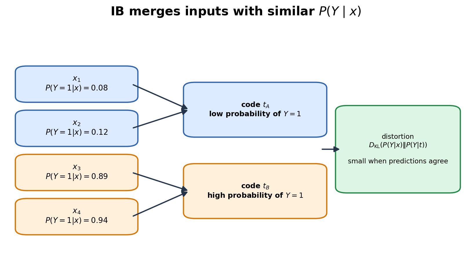
The final term does not depend on the encoder. IB is therefore a rate–distortion problem in which distortion measures damage to the prediction of $Y$, not a geometric distance between an input and its code.

This is one of the central results of the module:

Two inputs may share a code when merging them barely changes what can be predicted about the target.

If

$$I(T;Y)=I(X;Y),$$

then

$$I(X;Y\mid T)=0,$$

and the representation preserves all target information available in the input. In that predictive sense, it is sufficient for $Y$. IB seeks not merely a sufficient representation, but one that is as compact as possible among sufficient representations.

The self-consistent solution

For finite alphabets, a stationary point of the classical IB problem satisfies

$$P(t\mid x) = \frac{P(t)}{Z_\beta(x)} \exp \left[ -\beta D_{\mathrm{KL}} \bigl(P(Y\mid x)\|P(Y\mid t)\bigr) \right].$$

The form is familiar from Module 8. Base mass $P(t)$ is exponentially tilted toward codes with low predictive distortion.

The equation is self-consistent because:

• $P(t)$ depends on $P(t\mid x)$;
• $P(Y\mid t)$ also depends on $P(t\mid x)$;
• and $P(t\mid x)$ is computed from both of them.

Iterations related to Blahut–Arimoto find a consistent soft clustering. In a large neural network, the true $P(Y\mid x)$ is unknown, the spaces are enormous, and mutual information is inaccessible directly. The next step is therefore variational.

9.4. Variational Information Bottleneck: making IB trainable

The classical objective contains three inconvenient objects:

• the unknown true $P(Y\mid T)$;
• the aggregate representation distribution $P(T)$;
• high-dimensional mutual information terms that are hard to estimate.

VIB replaces each of them with a trainable probabilistic model.

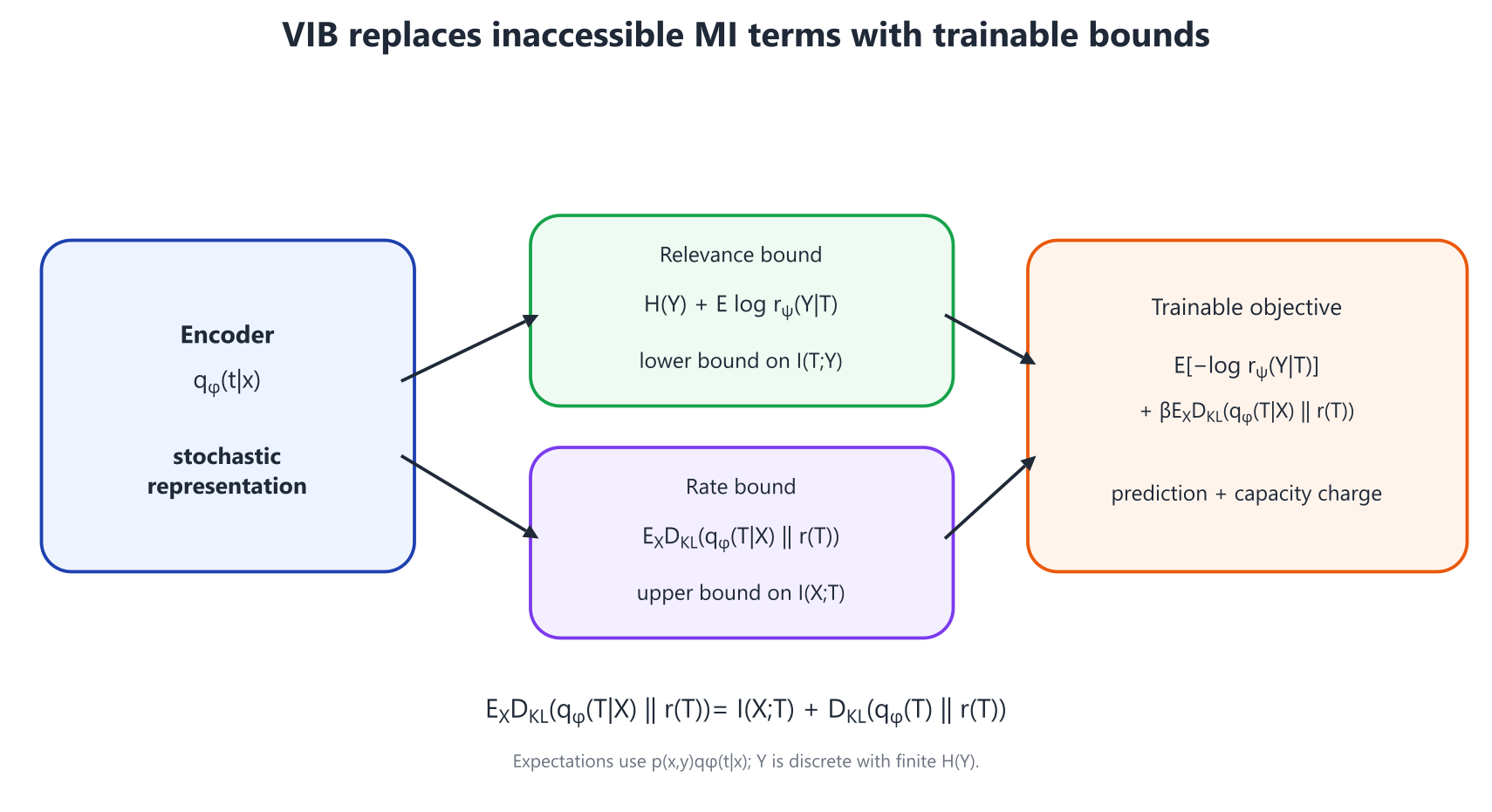
Let the encoder define a stochastic representation

$$q_\phi(t\mid x),$$

let a classifier define a variational decoder

$$r_\psi(y\mid t),$$

and choose a simple prior $r(t)$, such as $\mathcal N(0,I)$.

Relevance: the classifier supplies a lower bound

For any $r_\psi(y\mid t)$,

$$\begin{aligned} \mathbb E[-\log r_\psi(Y\mid T)] &= H(Y\mid T)\\ &\quad+ \mathbb E_T D_{\mathrm{KL}} \bigl( P_{Y\mid T} \|r_\psi(\cdot\mid T) \bigr)\\ &\ge H(Y\mid T). \end{aligned}$$

Hence

$$I(T;Y) =H(Y)-H(Y\mid T) \ge H(Y)+\mathbb E[\log r_\psi(Y\mid T)].$$

Cross-entropy is not literally $-I(T;Y)$. Subtracting it from $H(Y)$ provides a trainable lower bound on relevance. The better the decoder approximates the true $P(Y\mid T)$, the tighter the bound.

Rate: KL to a prior supplies an upper bound

Define the aggregate representation distribution

$$q_\phi(t) = \mathbb E_{X\sim P_X} [q_\phi(t\mid X)].$$

Then

$$\boxed{ \mathbb E_X D_{\mathrm{KL}} \bigl(q_\phi(T\mid X)\|r(T)\bigr) = I_q(X;T) + D_{\mathrm{KL}} \bigl(q_\phi(T)\|r(T)\bigr) }.$$

Therefore,

$$I_q(X;T) \le \mathbb E_X D_{\mathrm{KL}} \bigl(q_\phi(T\mid X)\|r(T)\bigr).$$

The average KL pays two bills:

1. information about the particular input that genuinely passes through $T$;
2. mismatch between the aggregate code distribution and the chosen prior.

If $r(t)=q_\phi(t)$, the second bill vanishes. With a simple fixed prior, it usually remains.

The trainable objective

A standard minimized VIB objective is

$$\boxed{ \mathcal J_{\mathrm{VIB}} = \mathbb E[-\log r_\psi(Y\mid T)] + \beta \mathbb E_X D_{\mathrm{KL}} \bigl(q_\phi(T\mid X)\|r(T)\bigr) }.$$

The first term pays for lost predictive information. The second charges for representation capacity.

For a diagonal Gaussian encoder,

$$q_\phi(t\mid x) = \mathcal N \bigl( \mu_\phi(x), \operatorname{diag}\sigma_\phi^2(x) \bigr),$$

with $r(t)=\mathcal N(0,I)$, the KL is analytic:

$$D_{\mathrm{KL}} \bigl(q_\phi(T\mid x)\|r(T)\bigr) = \frac12 \sum_j \left( \mu_j^2+\sigma_j^2-\log\sigma_j^2-1 \right).$$

This is already a familiar ML loss. Large $|\mu_j|$ is expensive; an excessively narrow conditional distribution is expensive too, because it can transmit a great deal of information about a specific $x$.

Sampling uses the reparameterization

$$T = \mu_\phi(X) + \sigma_\phi(X)\odot\varepsilon, \qquad \varepsilon\sim\mathcal N(0,I).$$

The stochasticity is more than a differentiation trick. It makes probabilistic capacity definable and controllable; the particular rate is finite when the chosen KL is finite.

What VIB actually guarantees

The positive result is already substantial: an ordinary trainable loss now has an exact information-theoretic origin, with one term for prediction and one for representation cost.

The precise objects are:

• the classification term is a variational bound on relevance;
• the KL term is an upper bound on $I(X;T)$;
• the rate gap depends on mismatch between $q_\phi(t)$ and $r(t)$;
• low rate is an inductive bias, not a universal certificate of generalization or robustness.

In experiments, it is therefore useful to log the terms separately: predictive NLL, average KL, the number of active dimensions, and held-out performance. A single scalar $\beta$ selects a trade-off, but it does not automatically explain where the model spent its information budget.

9.5. The VAE as a rate–distortion system

VIB preserves information about an external target $Y$. A VAE has no such target: the model must explain the observation $X$ itself through a latent variable $Z$.

The generative model is

$$p_\theta(x,z) =p(z)p_\theta(x\mid z),$$

and the encoder approximates the posterior:

$$q_\phi(z\mid x)\approx p_\theta(z\mid x).$$

For one observation,

$$\operatorname{ELBO}(x) = \mathbb E_{q_\phi(z\mid x)} [\log p_\theta(x\mid z)] - D_{\mathrm{KL}} \bigl(q_\phi(z\mid x)\|p(z)\bigr).$$

As shown in Module 4,

$$\log p_\theta(x) = \operatorname{ELBO}(x) + D_{\mathrm{KL}} \bigl(q_\phi(z\mid x)\|p_\theta(z\mid x)\bigr).$$

Thus the ELBO is both a trainable lower bound on log-likelihood and an exact variational-inference objective.

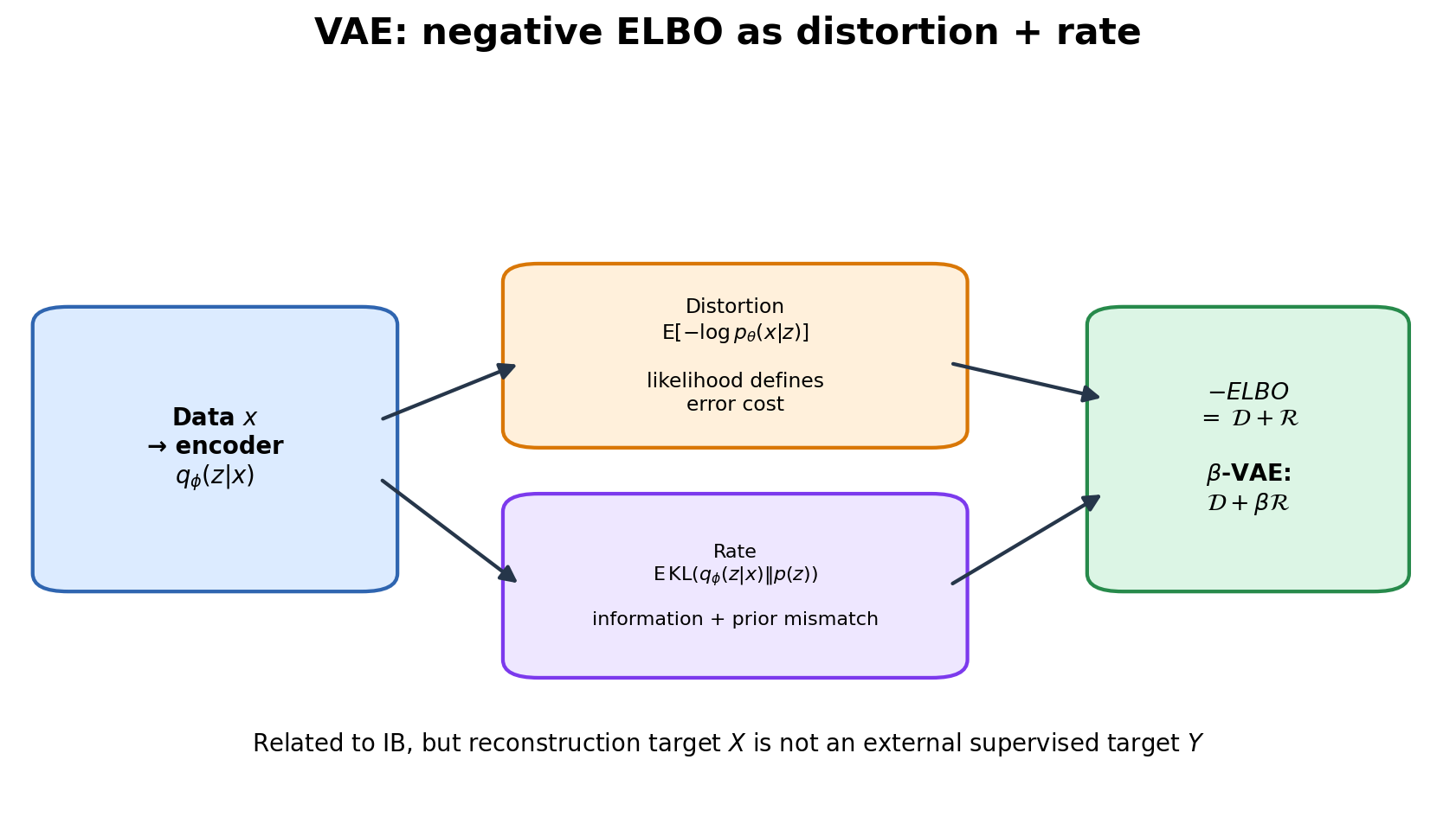
Averaged over data, the negative ELBO becomes

$$\boxed{ -\mathbb E[\operatorname{ELBO}] = \underbrace{ \mathbb E[-\log p_\theta(X\mid Z)] }_{\mathcal D\;\text{— distortion}} + \underbrace{ \mathbb E_X D_{\mathrm{KL}} \bigl(q_\phi(Z\mid X)\|p(Z)\bigr) }_{\mathcal R\;\text{— rate}} }.$$

It is worth pausing to read this formula in words:

A VAE pays for how hard the observation is to reconstruct from the latent and for how much information the latent consumes relative to the prior.

The decoder likelihood defines distortion

If

$$p_\theta(x\mid z) = \mathcal N \bigl( \mu_\theta(z), \sigma^2I \bigr)$$

with fixed $\sigma^2$, then

$$-\log p_\theta(x\mid z) = \text{const} + \frac{\|x-\mu_\theta(z)\|^2}{2\sigma^2}.$$

Distortion is proportional to MSE. The coefficient $1/(2\sigma^2)$ matters: changing the assumed noise changes the exchange rate between reconstruction and rate even when the explicit $\beta$ remains one.

A Bernoulli decoder yields binary cross-entropy. A categorical decoder yields a multiclass NLL. Choosing a likelihood means choosing the geometry of errors, not merely selecting an output layer.

Rate contains information and prior mismatch

Let

$$q_\phi(z) = \mathbb E_X[q_\phi(z\mid X)].$$

Then

$$\boxed{ \mathcal R = I_q(X;Z) + D_{\mathrm{KL}} \bigl(q_\phi(Z)\|p(Z)\bigr) }.$$

The VAE KL therefore pays for:

1. information about the particular object $X$;
2. mismatch between the aggregate code distribution and the prior used by the generative model.

The second term matters for generation and coding: the decoder must be able to obtain latents from the distribution declared as the prior.

VAE, $\beta$-VAE, and IB: shared geometry, different problems

A $\beta$-VAE minimizes

$$\mathcal D+\beta\mathcal R.$$

Larger $\beta$ penalizes use of the latent channel more strongly. Across well-optimized models, this usually shifts the operating point toward lower rate and higher distortion, although non-convex optimization does not guarantee perfect monotonicity across individual runs.

The conventions must not be mixed up:

• in $I(X;T)-\beta I(T;Y)$, larger $\beta$ protects relevance more strongly;
• in $\mathcal D+\beta\mathcal R$, larger $\beta$ penalizes rate more strongly.

A standard VAE is best understood as a variational rate–distortion system for generative modeling and reconstruction. It is related to IB through the same bottleneck mathematics, but it is not literally supervised IB: there is no external $Y$, and the usefulness of the latent is defined by $p_\theta(x\mid z)$.

Posterior collapse

A sufficiently powerful decoder may model $X$ well while barely using $Z$:

$$q_\phi(z\mid x)\approx p(z), \qquad \mathcal R\approx0.$$

This is posterior collapse. From the ELBO's perspective, the model has found a cheap solution: it stopped paying for the latent channel. From the perspective of a task that needs an informative latent, this is a failure.

Common ways to manage the regime include:

• KL warm-up;
• free bits, or a small free capacity per dimension;
• an explicit target capacity $C$ rather than immediate pressure toward zero;
• a less dominant decoder;
• a more expressive prior;
• monitoring active latent dimensions and achieved rate.

Disentanglement does not follow from one coefficient

A stronger rate penalty may encourage simpler and more factorized latents. The objective $\mathcal D+\beta\mathcal R$, however, does not force coordinates to align with the “true” factors of the data.

Without inductive assumptions about the data or architecture, or some weak supervision, unsupervised disentanglement is generally non-identifiable. A $\beta$-VAE is a useful capacity-control mechanism, not an automatic extractor of semantically correct axes.

Optional: IWAE

IWAE uses $K$ samples:

$$\mathcal L_K = \mathbb E \log \left[ \frac1K \sum_{k=1}^{K} \frac{p_\theta(x,z_k)}{q_\phi(z_k\mid x)} \right].$$

Under standard conditions,

$$\mathcal L_1\le\mathcal L_2\le\cdots\le\log p_\theta(x).$$

A tighter likelihood bound can improve density estimation, but it does not automatically yield a more interpretable or more useful representation. It also changes the encoder's gradient geometry, so “better bound” and “better latent” are different questions.

9.6. When rate becomes actual bits

In VIB and VAEs, “rate” has so far meant an information cost inside a probabilistic model. A file still requires a coder and a precise protocol—the same lesson as in Module 6.

Two cases are particularly instructive.

Learned lossy compression

A modern neural codec typically constructs:

1. a continuous latent $Y=g_a(X)$;
2. a quantized latent $\widehat Y$;
3. an entropy model $p_\psi(\widehat y)$;
4. a reconstruction $\widehat X=g_s(\widehat Y)$.

A typical objective is

$$\boxed{ \widehat R+\lambda\widehat D = \mathbb E[-\log_2p_\psi(\widehat Y)] + \lambda\,\mathbb E[d(X,\widehat X)] }.$$

If $p_\psi$ is then used by a compatible arithmetic or ANS coder, the first term has a literal interpretation as an expected bit count, up to finite-length, rounding, and metadata overhead.

A codec with a hyperprior sends both main and side latents:

$$\widehat R \approx \mathbb E \left[ -\log_2p(\widehat Z) -\log_2p(\widehat Y\mid\widehat Z) \right].$$

The hyperlatent adds its own bill but may improve prediction of $\widehat Y$ enough to reduce the total rate. This is a useful example of how adding a variable can improve compression rather than worsen it.

During training, hard rounding is usually replaced by a differentiable approximation such as uniform noise, a straight-through gradient estimate, or another surrogate. Evaluation must return to the true quantizer and a physical bitstream.

ELBO as codelength: bits-back

The VAE connection to coding can also be literal. Consider one observation $x$ and a latent $z$.

A naive code would pay

$$-\log p(z)-\log p_\theta(x\mid z).$$

The encoder, however, knows $q_\phi(z\mid x)$. In a bits-back scheme, some random bits are used to draw $z\sim q_\phi(z\mid x)$; after decoding, those bits can be recovered by encoding $z$ under $q_\phi(z\mid x)$ again.

The net length for the selected $z$ is

$$-\log p_\theta(x\mid z) -\log p(z) +\log q_\phi(z\mid x).$$

With base-2 logarithms, averaging over $q_\phi(z\mid x)$ gives exactly

$$-\operatorname{ELBO}(x).$$

The negative ELBO is therefore more than a convenient loss. Under a suitable bits-back implementation, it is the expected net codelength of the latent-variable model.

The practical protocol is more involved than the formula: it needs seed bits, a synchronized operation order, finite precision, and a stack-like coder such as ANS. Yet the mechanism explains why variational inference quality affects compression—a large variational gap means the code fails to recover as many bits as it could.

Quantizing LLM weights: the same discipline, not the same code

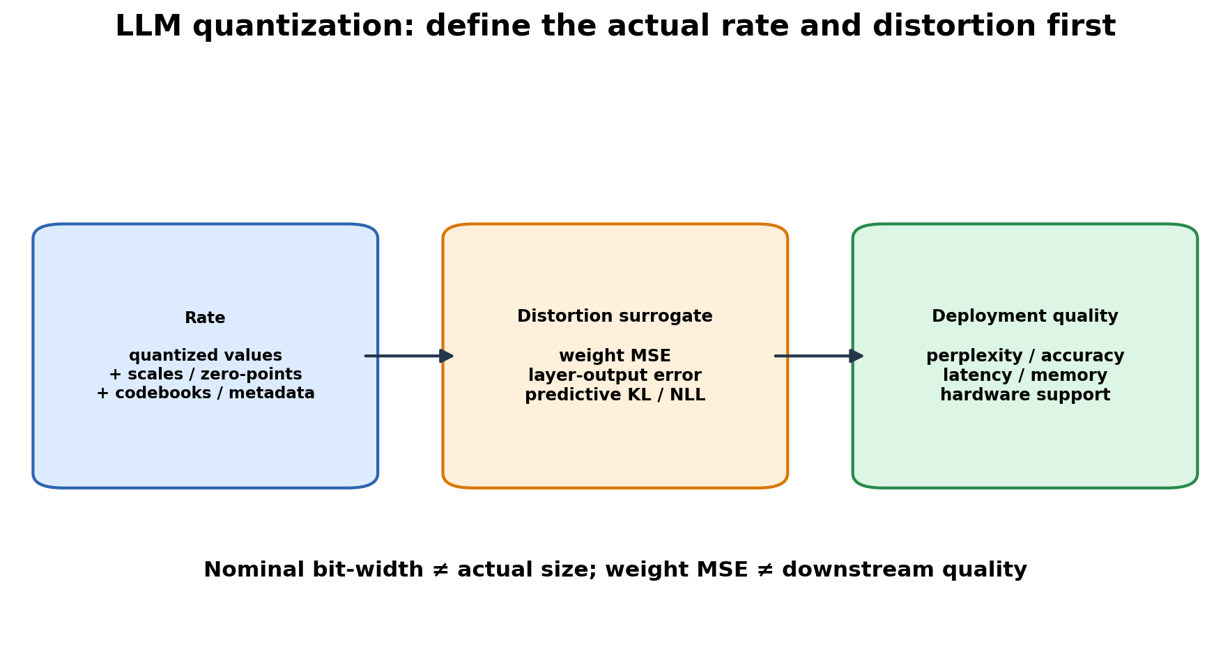
Let trained weights $W$ be replaced by $\widehat W$. The phrase “4 bits per parameter” specifies only nominal precision. The actual size may also include:

• group scales;
• zero-points;
• codebooks and indices;
• outliers retained at higher precision;
• alignment, packing, and headers.

Distortion must also be defined. Possibilities include

$$\|W-\widehat W\|_2^2,$$ $$\mathbb E\|WX-\widehat WX\|_2^2,$$ $$\mathbb E D_{\mathrm{KL}} \bigl( P_{\text{original}}(\cdot\mid c) \|P_{\text{quantized}}(\cdot\mid c) \bigr),$$

or an increase in NLL or downstream error.

The same weight MSE in two parameter-space directions can have radically different functional effects. Quantization methods therefore search for better distortion surrogates:

• GPTQ uses approximate second-order information for sequential error compensation;
• AWQ uses activation statistics to identify important channels;
• SmoothQuant uses an equivalent rescaling to move part of the quantization difficulty between activations and weights.

These methods fit naturally into rate–distortion language: they allocate a limited budget non-uniformly where errors are most costly. They do not prove that a Shannon $R(D)$ has been attained for a universal source of model weights.

9.7. Building an honest rate–distortion curve

One model at one value of $\beta$ or one bit-width is not a trade-off. It is a single point, and it may simply be poorly optimized.

A useful experiment constructs a series:

1. fix the training and evaluation distributions;
2. define rate precisely;
3. define distortion precisely;
4. sweep $\lambda$, $\beta$, capacity, or bit-width;
5. retain the non-dominated points—the empirical Pareto frontier;
6. measure latency, memory, and hardware cost separately.

The same words refer to different objects in different problems:

Before publishing a polished curve, ask four questions:

• Is rate measured per pixel, object, parameter, token, or latent coordinate?
• Are metadata and entropy-model parameters included?
• Is distortion evaluated on held-out data, and does it match the user's task?
• Does an average hide a small number of catastrophic errors?

There is also an engineering boundary: a smaller file does not guarantee faster inference. Awkward unpacking, unsupported precision, or additional memory traffic may erase the gain. Information theory supplies one axis; the deployed system adds a computational axis.

Rate–distortion is not the name of one metric. It is a discipline for specifying the problem.

9.8. The information plane: an objective or a description of training dynamics?

The Information Bottleneck as a normative principle is precise: we choose a stochastic map $P_{T\mid X}$ and optimize an explicit objective.

A stronger claim says something different: an ordinary deep network trained with standard SGD and no IB regularizer supposedly follows a characteristic trajectory in the plane

$$\bigl(I(X;T),I(T;Y)\bigr).$$

Early work proposed two phases:

1. fitting—information about labels increases;
2. compression—$I(X;T)$ falls while $I(T;Y)$ remains nearly stable.

It is an appealing story: the network first learns to predict and then forgets input detail. The debate around it proved more useful than the slogan because it forced a basic question: what exactly is plotted on the axes?

For a deterministic network $T=f(X)$, two regimes arise.

If $X$ is discrete, then

$$I(X;T)=H(T).$$

If the map is injective on the support,

$$H(T)=H(X),$$

so true mutual information need not decrease during training.

If $X$ is continuous and $T=f(X)$ is deterministic, the joint law often lies on a lower-dimensional set, and mutual information in the standard continuous formulation may be infinite.

To obtain a finite, changing quantity, an analyst adds noise, quantization, or binning. But this defines the MI of a particular noisy or quantized model, not an abstract “information in the layer.”

Saxe and coauthors showed that the observed compression phase depends on activation functions and the estimator. Goldfeld and coauthors clarified that earlier binning estimates could track geometric clustering of same-class representations even when they did not estimate the literal true MI of a deterministic layer.

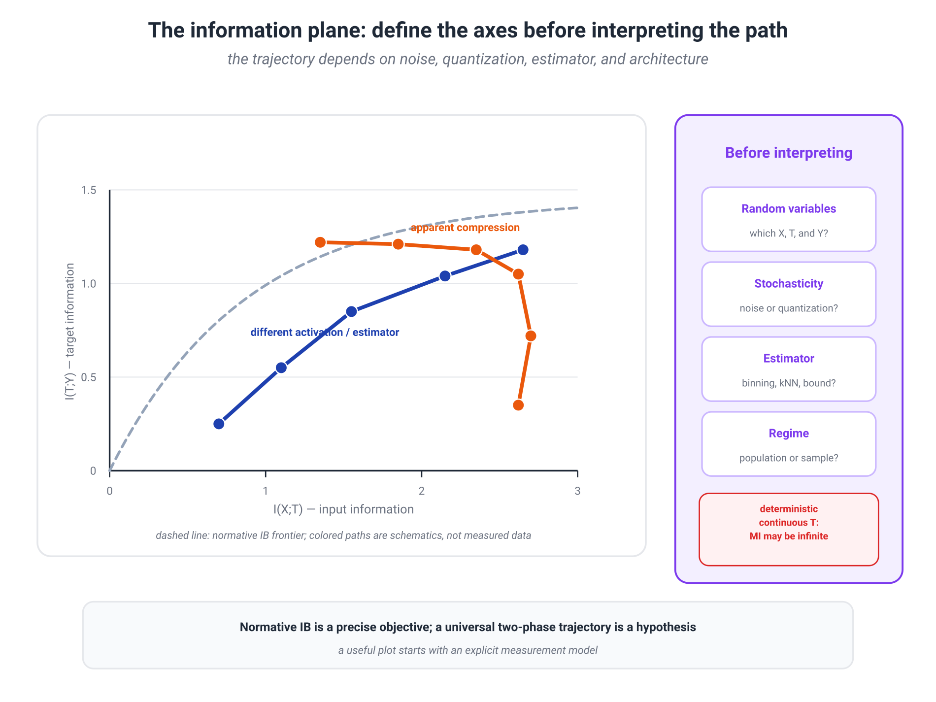
The right conclusion is not that information planes are forbidden, but that claims have levels:

• normative IB is a precise optimization problem;
• VIB is a specific trainable variational realization;
• the information plane of a noisy network is meaningful after noise and the estimator are defined;
• a universal spontaneous IB trajectory for all deep networks is an empirical hypothesis, not a consequence of DPI.

This is a recurring habit of the course: define the random variables and distributions first, and interpret the picture second.

9.9. Mathematical extension: I–MMSE and Gaussian noising

This section is not required for VIB or VAEs. It gives another exact bridge between retained information and reconstruction quality.

Rate–distortion theory asks how much information is needed for a specified MSE. The I–MMSE identity asks a local inverse question:

How quickly does mutual information grow when the SNR of a Gaussian observation is increased slightly?

Consider

$$Y_\gamma = \sqrt\gamma X+N, \qquad N\sim\mathcal N(0,1),$$

with $\mathbb E[X^2]<\infty$.

Define

$$\operatorname{mmse}(\gamma) = \mathbb E \left[ \left( X-\mathbb E[X\mid Y_\gamma] \right)^2 \right].$$

For mutual information measured in nats,

$$\boxed{ \frac{d}{d\gamma} I(X;Y_\gamma) = \frac12\operatorname{mmse}(\gamma) }.$$

For bits, the right-hand side is additionally divided by $\ln2$.

For every finite $\Gamma$,

$$I(X;Y_\Gamma) = \frac12 \int_0^\Gamma \operatorname{mmse}(\gamma)\,d\gamma.$$

The statement is literal: the area under the optimal reconstruction-error curve equals the information accumulated through the Gaussian channel.

The Gaussian example closes the loop

Let

$$X\sim\mathcal N(0,\sigma^2).$$

Then

$$\operatorname{mmse}(\gamma) = \frac{\sigma^2}{1+\gamma\sigma^2},$$

and

$$I(X;Y_\gamma) = \frac12\ln(1+\gamma\sigma^2).$$

Write the achieved reconstruction error as

$$D = \frac{\sigma^2}{1+\gamma\sigma^2}.$$

Then

$$1+\gamma\sigma^2 = \frac{\sigma^2}{D},$$

so

$$I(X;Y_\gamma) = \frac12\ln\frac{\sigma^2}{D}.$$

In bits, this is exactly the Gaussian rate–distortion function:

$$R(D)=\frac12\log_2\frac{\sigma^2}{D}.$$

Two parts of the module meet in one formula: optimal estimation error along a Gaussian channel reproduces the rate–distortion boundary of a Gaussian source.

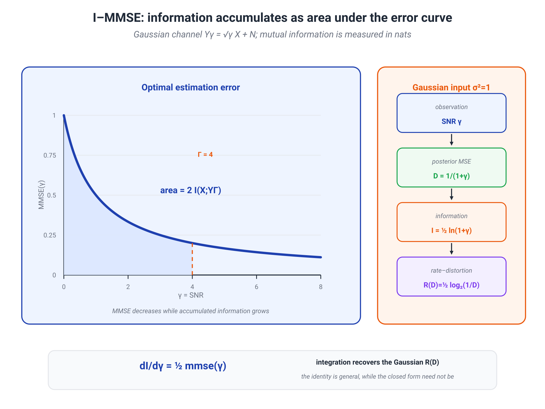
Why the infinite-SNR integral needs care

For discrete $X$ with finite entropy, one typically has

$$I(X;Y_\Gamma)\to H(X)$$

as $\Gamma\to\infty$.

For a non-degenerate absolutely continuous $X$, mutual information usually grows without bound. Therefore, without an additional renormalization, one cannot write

$$h(X) = \frac12 \int_0^\infty \operatorname{mmse}(\gamma)\,d\gamma.$$

For a standard Gaussian input, the integral diverges as $\tfrac12\ln(1+\Gamma)$ even though differential entropy is finite. Once again, a discrete intuition cannot be moved to the continuous case without checking the reference measure.

Connection to diffusion models

The forward noising process in a DDPM is

$$X_t = \sqrt{\bar\alpha_t}X_0 + \sqrt{1-\bar\alpha_t}\,\varepsilon, \qquad \varepsilon\sim\mathcal N(0,I).$$

After rescaling, this is a Gaussian channel with

$$\gamma_t = \frac{\bar\alpha_t}{1-\bar\alpha_t}.$$

For the true noised distribution, Tweedie's formula gives

$$\boxed{ \mathbb E[X_0\mid X_t=x_t] = \frac{ x_t + (1-\bar\alpha_t) \nabla_{x_t}\log p_t(x_t) }{ \sqrt{\bar\alpha_t} } }.$$

The exact score determines the posterior mean, the MSE-optimal denoiser. Score learning can therefore be read as learning a family of optimal reconstructors across noise levels.

I–MMSE alone, however, does not determine:

• the weighting of every diffusion training objective;
• a perceptually optimal noise schedule;
• the number of sampling steps;
• an equivalence between diffusion, flow matching, and IB.

Variational Diffusion Models connect a continuous-time variational bound to SNR and establish important schedule-invariance properties. That is additional structure from a particular probabilistic model, not an automatic consequence of I–MMSE alone.

9.11. What to carry forward

Information loss is useful only relative to a task. Differences that are irrelevant to a classifier may be essential to a reconstructor or to another target variable.

Rate–distortion theory gives a fundamental limit only after the source and the cost of error have been specified:

$$R(D) = \inf_{P_{\widehat X\mid X}:\ \mathbb E d\le D} I(X;\widehat X).$$

The Information Bottleneck makes distortion predictive:

$$d_{\mathrm{IB}}(x,t) = D_{\mathrm{KL}} \bigl(P(Y\mid x)\|P(Y\mid t)\bigr).$$

VIB turns inaccessible mutual information terms into a trainable objective, using a lower bound on relevance and an upper bound on rate.

A VAE is naturally read in rate–distortion coordinates:

$$-\operatorname{ELBO} = \text{distortion} + \text{rate}.$$

This makes VAEs relatives of IB, not the same optimization problem. The VAE has no external $Y$; its reconstruction likelihood defines what counts as useful information.

In an actual codec, rate must reach a bitstream. Latent NLL, a KL regularizer, nominal precision, and physical file size are related but distinct quantities.

An information plane is meaningful only after randomness and the estimator have been defined. Normative IB is a theorem and an objective; spontaneous IB dynamics in an ordinary network is an empirical hypothesis.

Finally, I–MMSE provides another reading of information: accumulated ability to reconstruct a signal optimally as SNR increases. For a Gaussian source, this connection returns exactly to the rate–distortion function and closes the module.

Primary sources

1. C. E. Shannon, Coding Theorems for a Discrete Source With a Fidelity Criterion.
2. N. Tishby, F. Pereira, W. Bialek, The Information Bottleneck Method.
3. A. Alemi et al., Deep Variational Information Bottleneck.
4. D. P. Kingma, M. Welling, Auto-Encoding Variational Bayes.
5. Y. Burda, R. Grosse, R. Salakhutdinov, Importance Weighted Autoencoders.
6. C. Burgess et al., Understanding Disentangling in $\beta$-VAE; F. Locatello et al., Challenging Common Assumptions in the Unsupervised Learning of Disentangled Representations.
7. J. Ballé et al., Variational Image Compression with a Scale Hyperprior; J. Townsend, T. Bird, D. Barber, Practical Lossless Compression with Latent Variables using Bits Back Coding.
8. Y. Blau, T. Michaeli, Rethinking Lossy Compression: The Rate-Distortion-Perception Tradeoff.
9. E. Frantar et al., GPTQ; J. Lin et al., AWQ; G. Xiao et al., SmoothQuant.
10. A. Saxe et al., On the Information Bottleneck Theory of Deep Learning; Z. Goldfeld et al., Estimating Information Flow in Deep Neural Networks.
11. D. Guo, S. Shamai, S. Verdú, Mutual Information and Minimum Mean-Square Error in Gaussian Channels.
12. J. Ho, A. Jain, P. Abbeel, Denoising Diffusion Probabilistic Models; D. P. Kingma et al., Variational Diffusion Models.