Module 7. Channel and capacity
How to read this module. Sections 7.1–7.7 form the classical core: the channel model, capacity, three basic examples, and both halves of the coding theorem. In §7.6, it is worth following at least the central random-coding count, because that is where the threshold becomes visible. The normal approximation at the end of §7.7 is intended for a second pass. Sections 7.8–7.10 bring the channel language back to ML: noisy labels, ECOC, learned communication, and LLMs.
7.1. Reliable communication through noise
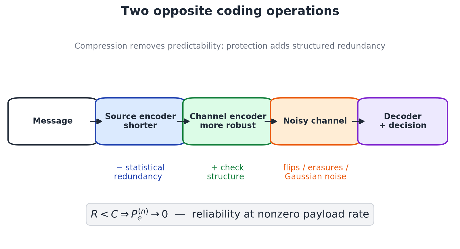
In Module 6, we tried to remove everything predictable from a message and represent it as compactly as possible. The new problem points in almost the opposite direction: the message must cross a medium that flips, erases, or corrupts symbols. Redundancy, which we had just worked to eliminate, suddenly becomes useful.
Imagine a binary channel that independently flips every transmitted bit with probability . If we send one thousand information bits without protection, the receiver will see about one hundred errors on average. The most obvious defense is repetition followed by majority voting. It helps, but it spends rate quickly: triple repetition carries only information bit per channel use and still does not eliminate error completely.
Shannon's result says something much stronger. This channel has capacity
bit per use. At every rate below , one can choose longer and longer block codes whose probability of error tends to zero. To first asymptotic order, one thousand information bits require at least
channel uses, not three thousand. This number does not yet promise a good short code of length —finite blocklength will need its own analysis. But it already breaks the naive choice between “rate” and “reliability.”
Noise need not be paid for by repeating each symbol. A good code separates entire messages in the space of long sequences so that typical noise does not confuse them.
This immediately separates two operations.
| Operation | What it does | Main criterion |
|---|---|---|
| Source coding | removes statistical redundancy | average description length |
| Channel coding | adds structured redundancy | error probability at a given rate |
The key word is structured. Appending random extra bits does not help. The additional symbols must keep codewords distinguishable under the distortions characteristic of the channel.
That is the content of the channel coding theorem: a given channel has a threshold . Below it, reliable communication is asymptotically achievable; above it, no code can make the error disappear. The second half matters just as much as the first: capacity is not a property of one coding algorithm, but a limit of the probabilistic channel model under its stated constraints.
For ML, this is not merely a decorative analogy. Annotator errors, noisy latent layers, quantized signals, wireless transmission of learned features, and coded class representations genuinely define channels once the input, output, and transition law are specified. Channel language is useful for LLMs as well, but there we will need to separate a precise model from a metaphor.
7.2. A discrete memoryless channel and a block code
To discuss a reliability limit, we first need a complete task. It has three parts: the channel, the codebook, and the decoder.
A discrete memoryless channel
A discrete memoryless channel (DMC) consists of
- a finite input alphabet ;
- a finite output alphabet ;
- a transition law
For channel uses, the conditional distribution factorizes:
“Memoryless” describes the noise conditional on the input sequence. It does not require the input symbols themselves to be independent. A useful codeword is usually highly structured across coordinates; that dependence is precisely where its protection comes from.
Two basic channels
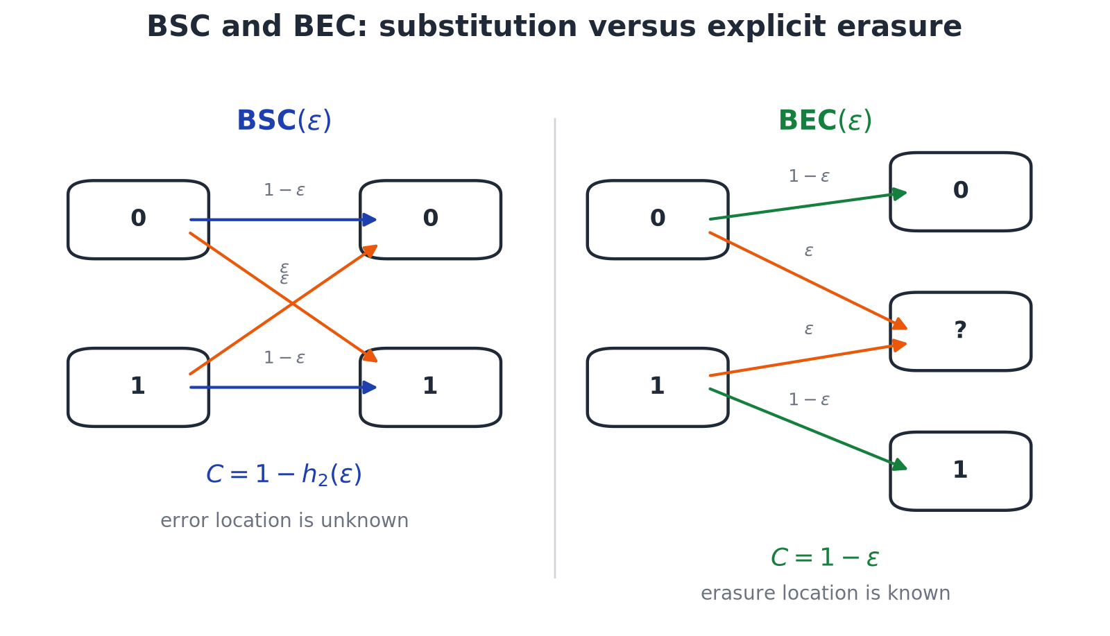
A binary symmetric channel (BSC) with crossover probability has transition matrix
Each transmitted bit is independently flipped with probability . The receiver sees or , but does not know where an error occurred.
A binary erasure channel (BEC) with erasure probability has output alphabet :
The receiver does not know the value of an erased bit, but does know its location. We will soon see how valuable that side information is.
A block code
Let the sender choose one of equiprobable messages:
A length- code consists of an encoder
and a decoder
The encoder sends the codeword
the channel produces , and the decoder returns
The average block error probability is
Sometimes the worst message must also be controlled:
Maximum error is at least average error and imposes a stronger requirement. For an ordinary DMC, the two criteria lead to the same capacity; moving to maximum error requires one extra expurgation step that removes the worst codewords.
The code rate
is measured in information bits per channel use. If , the code distinguishes messages and transmits bits of choice over uses.
A rate is achievable if there is a sequence of codes such that
Capacity is defined operationally as
So far, this tells us what quantity we want, but not how to calculate it. The next formula connects this engineering definition to the mutual information of Module 5.
A unit warning is also essential: bits per channel use are not bits per second. Physical throughput additionally depends on how many independent, or effectively independent, channel uses are available per second.
7.3. Capacity of a discrete channel
For a finite DMC with no additional input constraint, Shannon's theorem gives
The input distribution and the transition law induce the joint distribution
For a fixed , mutual information answers
How much information about the random input remains, on average, in one output under this way of using the channel?
Capacity asks a second question:
Which input distribution uses the channel best?
The distinction is easy to miss because both quantities have units of bits per use. But is an operating point under a chosen , whereas is the optimum over all admissible operating points.
The theorem has two halves.
- Achievability: for every , there are codes with .
- Converse: if , the error cannot tend to zero. For a DMC, the strong converse states that .
Mutual information therefore acquires an operational meaning. It is not only a measure of dependence between and : after optimizing the input, it becomes the highest reliable communication rate.
Reading the optimization over
Suppose an annotator confusion matrix is treated as a channel from a clean label to an observed label . In an actual dataset, the class distribution is fixed, so
measures the information preserved at those class frequencies. By contrast,
describes the best possible use of the same transition matrix. One number concerns the dataset; the other concerns the channel as a mathematical object.
A few consequences
For a finite DMC,
Capacity is zero if and only if all rows of the transition matrix are identical:
Then the output has the same distribution under every input and cannot distinguish messages.
If input symbols have different costs, capacity becomes
This line is especially important for continuous channels. Without a power or amplitude constraint, one could keep separating signals farther apart and obtain unbounded rates. The resource constraint is part of the problem definition, not an afterthought attached to the formula.
7.4. BSC, BEC, and the Z-channel
Three binary channels show why the single word “noise” is not enough. What matters is not only how often symbols are damaged, but also what structure of error the receiver observes.
Binary symmetric channel
Let . For a BSC, the output is also uniform and the conditional entropy is . Hence
Channel symmetry makes the uniform input optimal:
At ,
It is usually enough to consider . If , the receiver can flip every output and obtain an equivalent BSC with crossover probability . At the extreme , the channel again transmits one bit without loss: it deterministically maps to and to .
Binary erasure channel
Let . When a symbol is not erased, the input is known exactly; when it is erased, all the original uncertainty remains. Therefore
and
The maximum is attained at :
At , this is bit/use—substantially larger than the BSC with the same numerical parameter. The point is not that erasure is intrinsically “weaker.” A BEC tells the decoder where damage occurred; a BSC first forces the decoder to infer whether an error occurred at all.
An asymmetric Z-channel
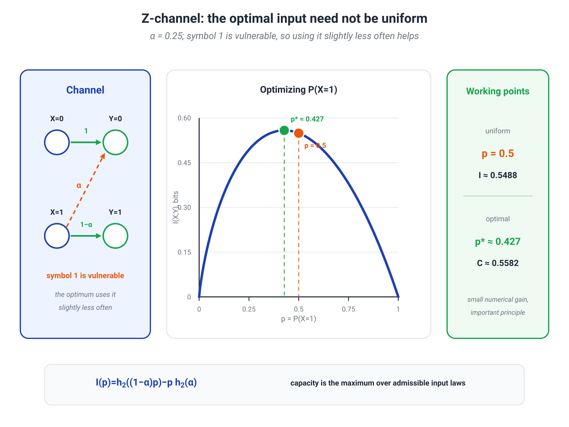
Now consider
Symbol passes without error, while changes to with probability . If
then
For , the maximum is attained approximately at
A uniform input gives slightly less:
The numerical difference is modest but the principle is important: the vulnerable symbol should be used less often. This is why the capacity formula optimizes over instead of silently assuming a uniform input.
For a general finite channel matrix, the optimum can be found with the Blahut–Arimoto algorithm; an implementation appears in the computational exercise.
7.5. The Gaussian channel and a power constraint
A discrete alphabet already limits how many signals can be distinguished. A real-valued channel has no such built-in ceiling, so its resource constraint must be stated explicitly.
Consider the discrete-time AWGN channel
where the noise is independent of the input and the average signal power satisfies
Capacity per real channel use is
bit/use. The optimal input is Gaussian:
The mechanism behind the formula is direct. Since ,
The noise entropy is fixed. Under variance , output entropy is maximized by a Gaussian distribution, and a Gaussian input makes the output Gaussian, achieving the bound.
For a continuous-time channel of bandwidth Hz, average signal power , and total noise power in that band, the Shannon–Hartley formula is
bit/s. The first formula is in bits per real channel use; the second is in bits per second. Their shared logarithm does not make the units interchangeable.
What the curve says
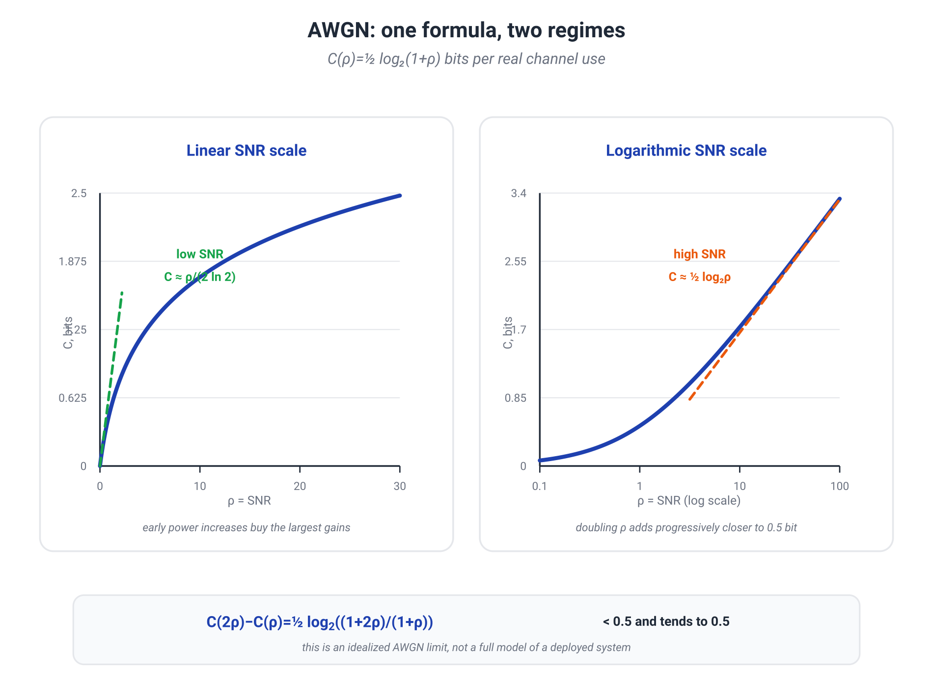
Let the signal-to-noise ratio (SNR) be . Then
- at low SNR, ,
- at high SNR, ,
At low SNR, extra power raises rate almost linearly. At high SNR, returns become logarithmic. The exact gain from doubling SNR is
It is below bit/use and approaches only at high SNR. Thus “doubling power buys half a bit” is a useful high-SNR approximation, not an identity over the entire curve.
The formula is a limit for an idealized model. A real system adds fading, interference, finite constellations, hardware constraints, latency, protocol overhead, and finite blocklength. A claim of operating “near the Shannon limit” is incomplete until it says which model and which error criterion define that limit.
7.6. Why random coding achieves
We have now reached the most surprising part of the theorem. To prove that a good code exists, Shannon did not begin with an ingenious explicit construction. He drew the entire codebook at random and bounded its average error.
This is one of those cases where a random object is easier to analyze than the best concrete object. If the average error over an ensemble of random codebooks tends to zero, at least one deterministic codebook performs no worse than the average.
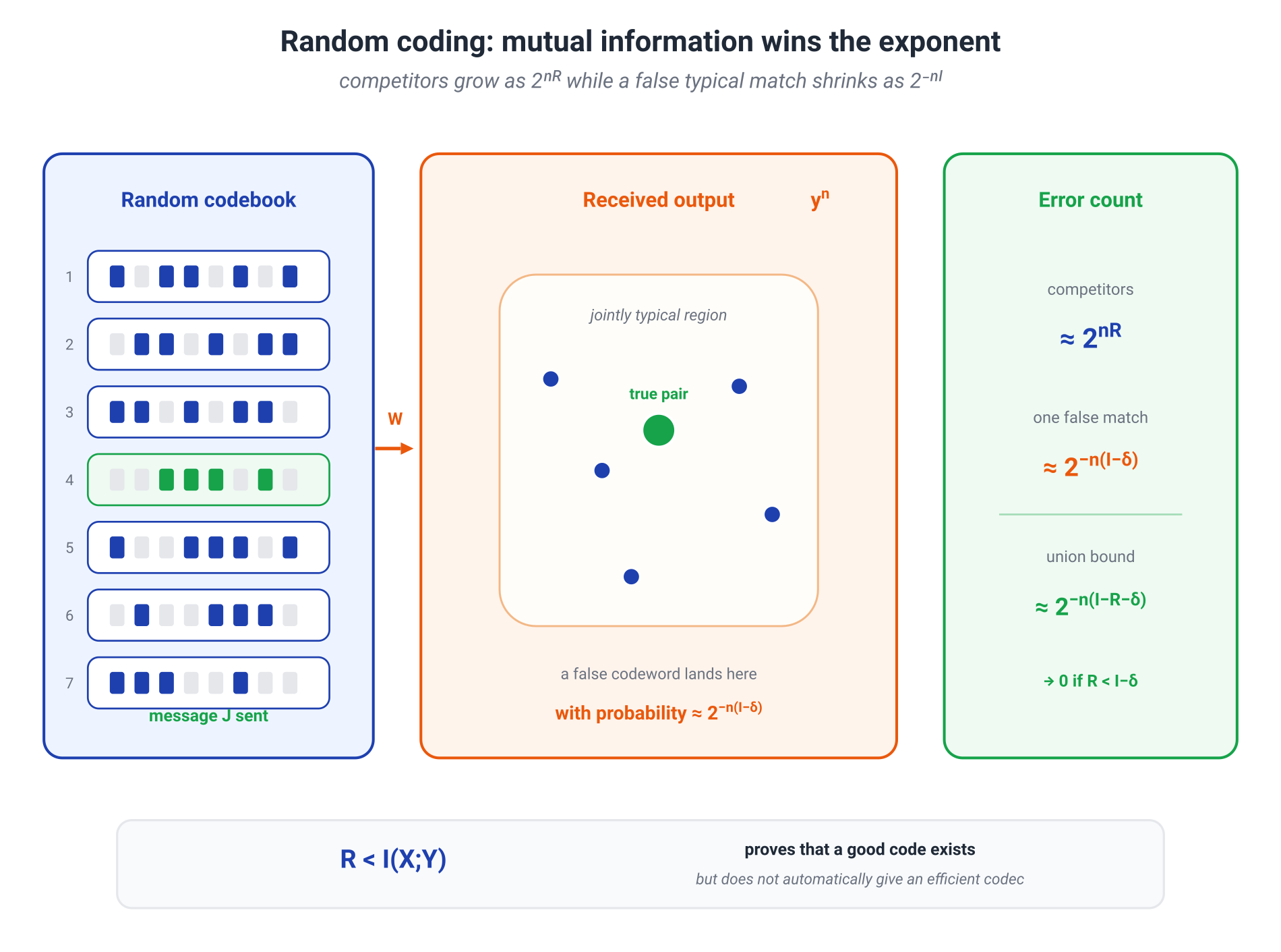
The whole count can first be seen in one line. A codebook contains about codewords. For a fixed wrong codeword, the chance of looking plausible next to the received output is of order . The total false-match risk is therefore of order
If , the number of competitors grows more slowly than the probability of a false match decays. That balance is the threshold.
Now let us state the argument precisely. Fix an input distribution and a rate
Let be the output distribution induced by and the channel.
Step 1. A random codebook
For each message , with
generate a codeword independently:
Step 2. Information density
For one input-output pair, define the information density
Its mean under the joint distribution is mutual information:
For a memoryless channel,
The law of large numbers gives, for the true pair,
Step 3. A threshold decoder
The decoder looks for the unique message such that
An error has two possible causes.
- The true pair misses the threshold. Its probability tends to zero by the law of large numbers.
- Some wrong codeword crosses the threshold.
For , the codeword is independent of . Under the product distribution ,
Markov's inequality gives
There are about wrong codewords, so a union bound yields
Choose so that
Both error terms then vanish. Since this holds for any fixed , optimizing proves achievability of every rate below
What the argument has established
First, it proves the existence of a deterministic code: a small ensemble-average error implies that some realization is good. More strongly, when the ensemble-average error vanishes, the fraction of codebooks with substantially larger error also vanishes under a suitable threshold. Good books are not isolated needles in the asymptotic ensemble.
Second, the argument explains why mutual information appears. It controls the exponent with which an unrelated codeword can masquerade as compatible with the output.
But an existence proof is not yet a convenient codec. A random book contains on the order of words, is expensive to store, and requires exponential brute-force decoding. Practical families—LDPC, turbo, and polar codes—supply structure and efficient decoders. The theorem first showed that there was something worth finding; coding theory then learned how to find it constructively.
7.7. Converse and finite blocklength
Achievability asks what can be done below . The converse sets a limit on every possible code: above , reliability cannot be restored by a cleverer encoder or decoder.
A short converse through Fano's inequality
Let be uniform over messages, with rate
Fano's inequality gives
Also,
The last line uses memorylessness:
Therefore
When , the right-hand side remains positive for large , so error cannot tend to zero. This is the weak converse.
For a DMC, the strong converse goes further: at a fixed ,
Above capacity, the channel does not merely enter a “slightly worse” regime. As blocklength grows, it almost entirely loses the ability to distinguish messages reliably at that rate.
Why is not yet an engineering answer
Capacity is a first-order asymptotic result. A real system specifies the triple
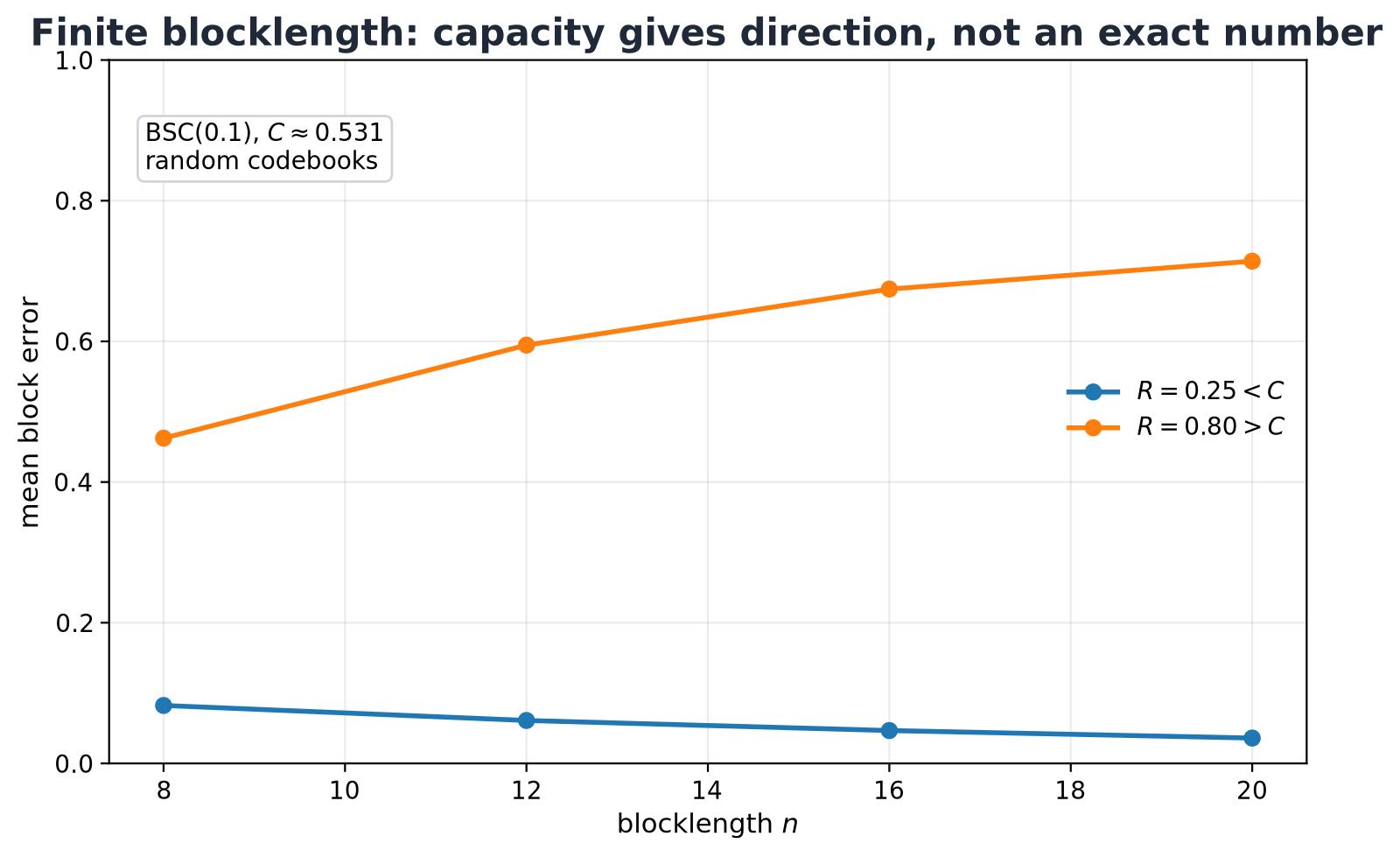
where is blocklength, is rate, and is the target error probability. At short blocklength, a rate below may still have large error. A substantial engineering problem lies between “asymptotically possible” and “works under a 10 ms latency budget.”
Mathematical deepening: the normal approximation
For many regular channels, the maximal rate at blocklength and target error is approximately
where is the channel dispersion and is the inverse Gaussian tail function.
Capacity sets the center, while captures fluctuations of information density and therefore the price of a short block. The higher the required reliability and the smaller , the farther the operating rate must back off from .
7.8. Noisy labels as a channel
We can now move the same structure from a communication link into a dataset. Let be a clean label and the label recorded after an annotator or an automated corruption pipeline. Under class-conditional noise, the transition is described by
This is a literal probabilistic channel
If the features influence the observed label only through the clean label, then
is a Markov chain, and data processing gives
A noisy label cannot retain more information about the input than a clean label. The amount lost, however, depends on the full transition matrix and the class distribution—not only on a single error rate.
Symmetric -class noise
Suppose a label remains correct with probability and, on an error, is replaced uniformly by one of the other classes:
For uniform , the output is uniform as well, so
This channel is weakly symmetric, so the uniform input is capacity-achieving and the same expression is its capacity.
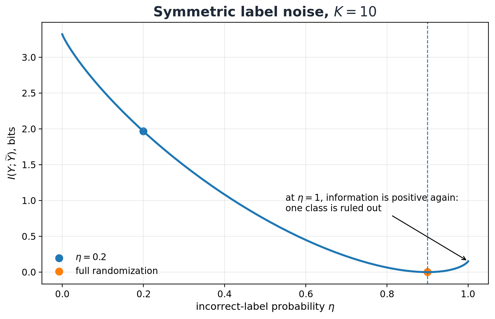
For and ,
out of the original bits.
The most interesting point is not but
Here every row becomes uniform and all information disappears. At , annotator accuracy is zero, but the recorded label still conveys one reliable fact: the true class is different from it. Thus
For , about bit remains. This is a clean example of why accuracy and mutual information answer different questions: a systematically wrong signal can still be fully or partially invertible.
Where the noise matrix stops being enough
Real annotation errors often depend on the instance , on the annotator, on ambiguity, and on the filtering pipeline. A single class-conditional matrix cannot represent all of those mechanisms.
When is known, it can be used for forward or backward loss correction. But inverting an ill-conditioned matrix amplifies statistical noise, and an estimated contributes its own error. Channel information loss, identifiability of the transition matrix, and numerical stability of correction are three separate problems.
7.9. Channel coding inside ML: ECOC and DeepJSCC
In this section, “code” is no longer only an analogy. In both constructions, an encoder, a channel, and a decoder are part of the algorithm itself.
Error-correcting output codes
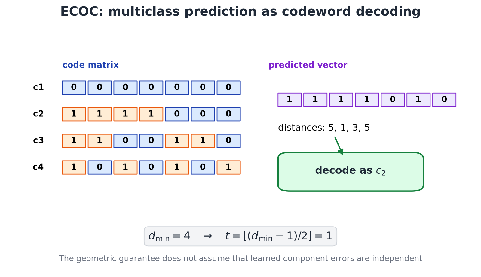
In error-correcting output codes (ECOC), each of classes receives a codeword
Each column of the code matrix defines a binary task, so the learner trains binary classifiers. Their outputs form a predicted word , and prediction selects the nearest class codeword.
If the minimum Hamming distance between codewords is , an ideal nearest-codeword decoder corrects up to
bit errors. The geometry is exactly the geometry of channel coding: error balls around different classes must not overlap.
In classification, however, the “error channel” is rarely an independent BSC. Binary classifiers share data, their errors are correlated, columns have different difficulty, and the error probability depends on . A large supplies a useful geometric margin, but not a complete statistical guarantee.
Learned joint source-channel coding
A classical digital system often separates three stages:
- source compression;
- error protection;
- mapping coded symbols into a physical signal.
In joint source-channel coding (JSCC), the full mapping is optimized jointly for a distortion measure and a channel model. In DeepJSCC, a neural encoder, a differentiable channel layer, and a neural decoder form
The parameters minimize reconstruction or task loss. In the original image experiments, DeepJSCC outperformed the chosen separation-based baselines in several low-SNR and low-bandwidth regimes, and its quality degraded smoothly under SNR mismatch rather than showing a sharp digital cliff.
This does not overturn the source-channel separation theorem. Under standard stationary models, asymptotically long blocks, and matched criteria, separate coding can be optimal. If channel uses are available per source symbol, the distortion condition is ; writing assumes and compatible units. DeepJSCC is attractive precisely where the practical problem departs from that ideal asymptotic setting: blocks are short, latency is constrained, the channel model may be mismatched, and quality is measured by continuous distortion rather than only exact recovery of bits.
7.10. An LLM as a channel: a precise model and the limits of the analogy
The word “channel” also arises naturally around language models. The useful move is not to reject the analogy, but to start with a version in which it is mathematically exact.
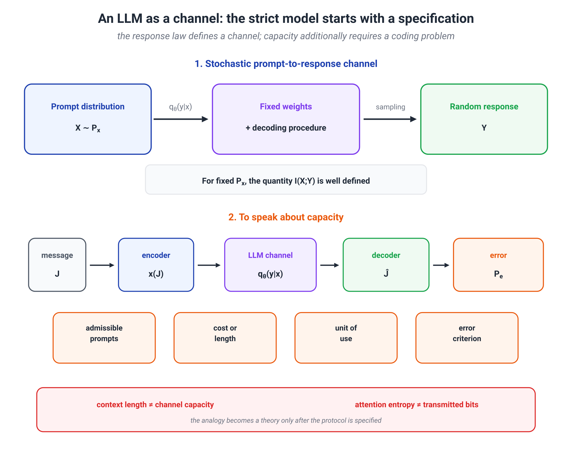
A channel from prompt to response
Fix the model weights, the context-construction rules, and the generation algorithm. Let be a random prompt and the generated response. Then
is a conditional output distribution and therefore defines a stochastic channel from to . Under a fixed prompt distribution, one can compute
With deterministic decoding, the channel simply becomes a deterministic map. With temperature sampling, top-, or another randomized procedure, those rules are part of the transition law.
To discuss capacity, we must add an operational coding task. For example, a sender chooses a message , encodes it as an admissible prompt of at most tokens, the model generates a response, and a decoder tries to recover . Only after specifying the prompt set, cost, unit of channel use, and error criterion does “maximum rate” become a precise quantity.
Such an experiment can be defined. But it measures the capacity of a particular prompt–model–response protocol, not a universal number attached to the Transformer architecture outside a task.
Context length as a resource
A context window of tokens is a real resource: it constrains input volume and computational cost. But the token count does not directly determine the number of reliably transmitted bits.
To turn window length into a channel quantity, one would need to specify
- the prompt distribution and admissible prompt set;
- the cost of different tokens or sequences;
- the response transition distribution;
- an encoder and decoder for messages;
- an error criterion;
- the role of knowledge already stored in model parameters.
Without these pieces, context length remains a resource size rather than a Shannon capacity.
Lost in the Middle showed that retrieval quality can depend strongly on the location of relevant evidence: in the studied tasks, models often used the beginning and end of a long context more effectively than its middle. This is an important empirical property of specific models and protocols. It does not follow automatically from DPI or from an abstract “window capacity”; its mechanism depends on architecture, positional encoding, training, and task design.
RAG changes the protocol before the model sees the input: a retriever selects a small set of evidence rather than placing an entire corpus into the prompt. The practical gain can be described as saving context budget and reducing competition from irrelevant passages. There is no need to call it an automatic increase in capacity—the more precise statement is already strong enough.
What attention weights measure
A row of attention weights
sums to one and therefore resembles a probability distribution. But it is a set of mixing coefficients over values, not a transition law from an input token to an output message. The layer output also depends on value vectors, multiple heads, the residual stream, and subsequent nonlinearities.
The entropy
has a clear local meaning: it describes how concentrated the routing weights are across keys. Low entropy means that mass is focused on a few positions; high entropy means it is spread more broadly. By itself, it is not the number of transmitted bits, causal influence, or the importance of a token to the final answer.
Chain of thought
Chain of thought (CoT) increases the number of generated tokens, the amount of externally represented intermediate state, and test-time compute. That can improve performance on difficult tasks. A channel metaphor—“the model receives more sequential uses of an external scratch medium”—may be a useful research intuition. It is not yet a theorem that CoT raises the model's Shannon capacity. Module 13 will return to this boundary in detail.
7.11. Formalizing a channel in an ML system
Channel language is most useful not when it produces a striking metaphor, but when it forces us to specify the experiment. Before computing MI or capacity, it helps to fill in a short specification.
| Element | Question |
|---|---|
| Input | Which random variable is transmitted? |
| Output | What does the receiver or next model observe? |
| Transition law | Where does randomness enter, and how is defined? |
| Constraint | What is limited: power, length, tokens, bits, or latency? |
| Code and decoder | How are messages mapped to inputs and recovered? |
| Criterion | Block error, MSE, top-1 accuracy, or semantic utility? |
| Regime | Fixed or asymptotics? Actual or maximization over ? |
Compare two settings.
| System | What is precisely defined | Which question can be asked |
|---|---|---|
| Noisy labels | , , and transition matrix | actual ; after optimizing class frequencies, the matrix capacity |
| LLM with fixed sampling | prompt , response , law | under a prompt distribution; capacity only after a coding task and cost are specified |
Two distinctions are worth carrying forward:
and
This is not a ban on analogies. It is how they become productive: first identify which part of the construction is a genuine channel, then mark clearly where the heuristic begins.
7.13. Conclusion
In Module 6, a probabilistic model became a bill in bits. In Module 7, mutual information acquired a second operational meaning: after optimizing the input, it gives the limiting reliable communication rate through noise.
A complete construction surrounds the short formula.
- The channel specifies a transition law and a resource constraint.
- The codebook maps messages into long, well-separated sequences.
- Below , random coding proves the existence of codes with vanishing error.
- Above , the converse forbids reliable communication for every code.
- At finite , capacity alone is not enough: target error and channel dispersion matter.
The main conceptual shift is that noise stops being a local defect that must be repaired one symbol at a time. A code acts on the geometry of the whole block. Individual channel uses still make errors, yet the complete message can remain reliably distinguishable.
For ML, this idea has two levels. In noisy labels, ECOC, and DeepJSCC, the channel is part of a precise model or algorithm. In discussions of context, attention, and CoT, channel language is usually a disciplined analogy. In both cases the same question is useful: can we explicitly write the input, output, transition law, resource constraint, and decoding task?
This completes the classical Shannon core. Source coding removes predictable redundancy; channel coding adds redundancy designed to survive noise; mutual information connects both sides to exact limits.
Module 8 moves from describing sources and channels to a normative question: which distribution should we choose when only constraints are known? The answer will be the maximum-entropy principle.
Primary sources and further reading
- C. E. Shannon, A Mathematical Theory of Communication, 1948.
- T. Cover, J. Thomas, Elements of Information Theory, 2nd ed., 2006, Chapters 7–9.
- Y. Polyanskiy, Y. Wu, Information Theory: From Coding to Learning, 2025, chapters on channel coding and finite blocklength.
- Y. Polyanskiy, H. V. Poor, S. Verdú, Channel Coding Rate in the Finite Blocklength Regime, 2010.
- R. Blahut, Computation of Channel Capacity and Rate-Distortion Functions, 1972; S. Arimoto, An Algorithm for Computing the Capacity of Arbitrary Discrete Memoryless Channels, 1972.
- G. Patrini et al., Making Deep Neural Networks Robust to Label Noise: A Loss Correction Approach, 2017.
- T. Dietterich, G. Bakiri, Solving Multiclass Learning Problems via Error-Correcting Output Codes, 1995.
- E. Bourtsoulatze, D. B. Kurka, D. Gündüz, Deep Joint Source-Channel Coding for Wireless Image Transmission, 2019.
- N. F. Liu et al., Lost in the Middle: How Language Models Use Long Contexts, 2024.
- S. Jain, B. C. Wallace, Attention is not Explanation, 2019; S. Wiegreffe, Y. Pinter, Attention is not not Explanation, 2019.