Module 8. Maximum entropy, exponential models, and KL regularization

How to read this module. The main route is §§8.1–8.9. Sections 8.1–8.5 build the MaxEnt principle from the modeling problem to conditional log-linear models; §§8.6–8.9 show the same variational mechanism in softmax, energy-based models, and LLM post-training. Section 8.10 is a self-contained mathematical deepening on exponential families, their main distributions, and sufficient statistics and can be saved for a second pass.

8.1. From partial knowledge to a distribution

Until now, a distribution usually appeared in the statement of the problem. We were given $P$ and computed its entropy; given $P$ and $Q$, we evaluated KL; given a channel, we studied its capacity. The distribution itself must now become the answer.

Consider an ordinary six-sided die. We have not observed its rolls, but we know that its mean is $4.5$. That is plainly insufficient to recover all six probabilities. For example, both

$$q_A=(0,0,0,\tfrac12,\tfrac12,0)$$

and

$$q_B=(0,0,\tfrac14,\tfrac14,\tfrac14,\tfrac14)$$

have mean $4.5$. Infinitely many other distributions lie between them. The constraint cuts down the simplex but does not select a single point.

This situation appears throughout ML.

• We know empirical feature averages and want a conditional class distribution.
• A network has produced logits, and we need to turn a system of scores into probabilities.
• We have a reference policy and a reward function; we want to improve behavior without destroying everything the model learned before.
• An energy-based model can score states but still has to reconcile those scores into one normalized distribution.

In every case, part of the structure is known, while the complete probability law must still be filled in.

The maximum entropy principle (MaxEnt), formulated by Edwin Jaynes as a rule of inference from incomplete information, gives a simple answer: among the distributions satisfying the explicitly stated constraints, choose the one with largest entropy.

On a finite state space,

$$q^* = \arg\max_{q\in\Delta} H(q) \quad\text{subject to}\quad \mathbb E_q[f_j(X)]=\mu_j.$$

The substance of the principle is not the slogan “choose the most random distribution.” It is a more careful discipline:

Do not introduce distinctions among admissible states for which the problem statement provides no basis.

If a reference distribution $m$ is already available, the question changes. We should not return to uniformity; we should modify the reference only as much as the new constraints require. This gives the relative form of MaxEnt:

$$\boxed{ q^* = \arg\min_{q\in\mathcal C} D_{\mathrm{KL}}(q\|m) },$$

where $\mathcal C$ is the set of distributions compatible with the known moments. If $m$ is uniform on a finite set, then

$$D_{\mathrm{KL}}(q\|m) = -H(q)+\log|\mathcal X|,$$

so minimum KL and ordinary MaxEnt have the same solution.

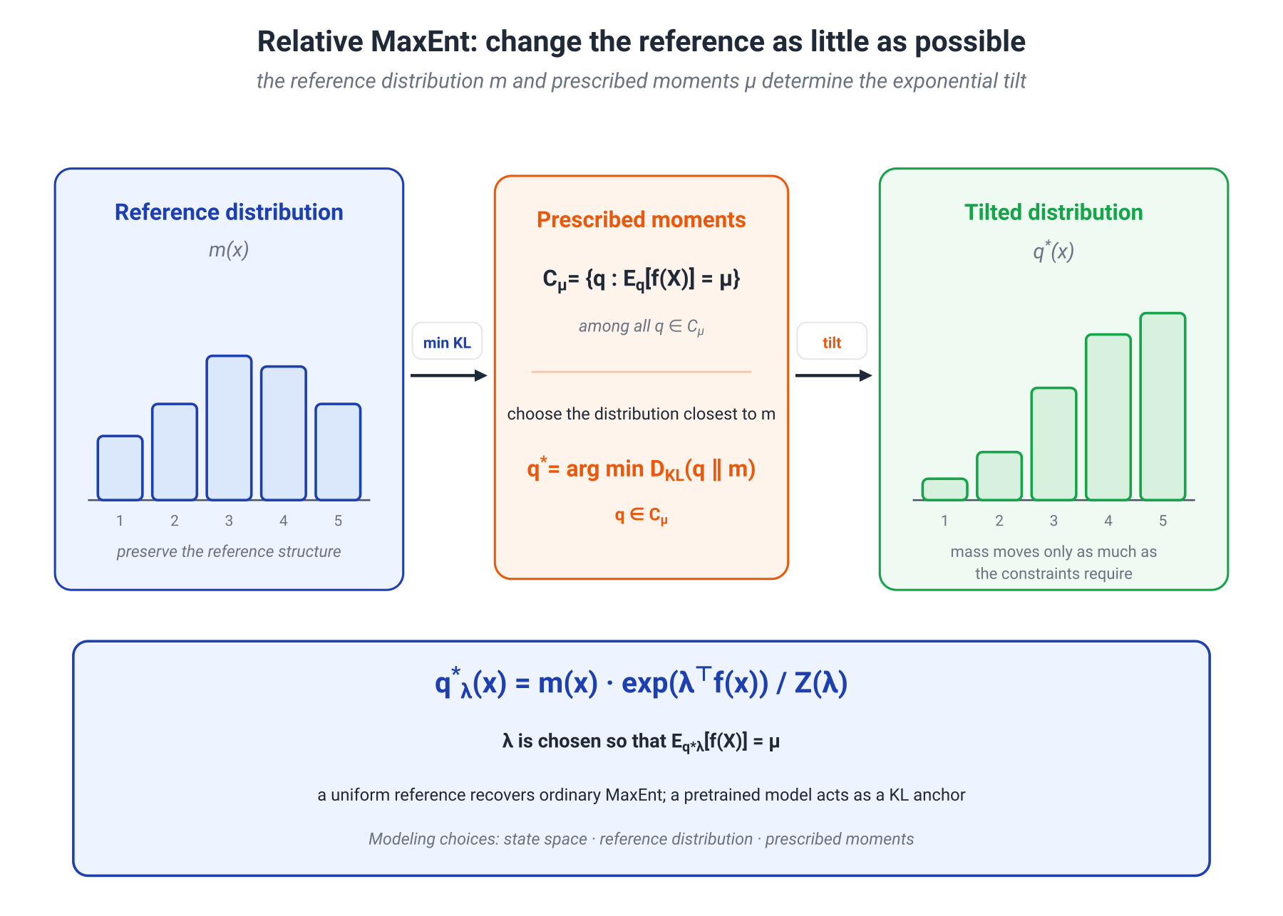
This relative formulation is especially useful in ML. The reference can be a pretrained language model, a prior distribution, an earlier policy, or a natural measure on the state space rather than an abstract uniform law.

Before deriving anything, however, three modeling choices must be named explicitly.

1. State space. What counts as one elementary outcome: a success count, a binary configuration, a class, or an entire token sequence?
2. Reference. Relative to which distribution or measure is departure being assessed?
3. Constraints. Which averages are actually known, and why are they the relevant ones?

MaxEnt does not guess the “true distribution” beyond these choices. It does something more modest and more useful: once the model of the problem is fixed, it removes arbitrariness from the completion.

One construction will recur throughout this module:

$$\text{reference} \quad\xrightarrow{\text{exponential tilt}}\quad \text{new distribution}.$$

In MaxEnt, the tilt is determined by moment constraints. In softmax, by logits and temperature. In an energy-based model, by negative energy. In a KL-regularized policy, by reward relative to a reference model. These are not four names for one theorem; they are four optimization problems whose optima are built by the same mathematical operation.

8.2. Exponential tilting and information projection

Consider a finite space $\mathcal X$ and a strictly positive reference

$$m(x)>0, \qquad \sum_xm(x)=1.$$

Suppose the means of functions $f_1, \ldots,f_k$ are known:

$$\mathbb E_q[f_j(X)]=\mu_j, \qquad j=1, \ldots,k.$$

We solve

$$\min_qD_{\mathrm{KL}}(q\|m)$$

subject to normalization and these linear constraints.

Lagrange-multiplier derivation

The Lagrangian can be written as

$$\begin{aligned} \mathcal L(q,\lambda,\nu) &= \sum_xq(x)\log\frac{q(x)}{m(x)}\\ &\quad- \lambda^\top \left( \sum_xq(x)f(x)-\mu \right) + \nu\left(\sum_xq(x)-1\right). \end{aligned}$$

At an interior solution $q(x)>0$,

$$\frac{\partial\mathcal L}{\partial q(x)} = \log\frac{q(x)}{m(x)}+1-\lambda^\top f(x)+\nu=0.$$

Rearranging and reading the result on the log-probability scale gives

$$\log q(x)-\log m(x) = \lambda^\top f(x)-\log Z(\lambda).$$

The constraints change log probability linearly. Exponentiating yields

$$\boxed{ q_\lambda(x) = \frac{m(x)\exp\bigl(\lambda^\top f(x)\bigr)} {Z(\lambda)} },$$

where

$$Z(\lambda) = \sum_xm(x)\exp\bigl(\lambda^\top f(x)\bigr)$$

is the partition function.

That is the entire mechanism of exponential tilting. The reference retains the original relative mass of states, while $e^{\lambda^\top f(x)}$ amplifies or suppresses it according to the constraints. With a uniform reference,

$$q_\lambda(x)\propto e^{\lambda^\top f(x)}.$$

The sign convention depends on the language of the problem. Statistics often uses a positive score $\lambda^\top f(x)$; physics introduces an energy $E(x)$ and writes $q(x)\propto e^{-\beta E(x)}$. The distribution is the same—the interpretation of the function in the exponent changes.

The partition function as a computational object

Let

$$A(\lambda)=\log Z(\lambda).$$

Then

$$\boxed{ \nabla A(\lambda) = \mathbb E_{q_\lambda}[f(X)] }$$

and

$$\boxed{ \nabla^2A(\lambda) = \operatorname{Cov}_{q_\lambda}(f(X)) \succeq0 }.$$

These two lines turn an elegant distributional form into a working method. To satisfy the constraints, solve

$$\nabla A(\lambda)=\mu.$$

The gradient reports the current model moments, and the Hessian describes how they change with the parameters. Because the Hessian is a covariance matrix, $A$ is convex. If the features are linearly redundant, the parameter $\lambda$ may not be unique; after redundant directions are removed, the corresponding convexity is strict.

The form should already look familiar. In softmax, $A$ becomes logsumexp; in an exponential family, it is the log-partition function; in a KL-regularized policy, it becomes a soft value of the reference policy. The same function both normalizes the distribution and stores its moments in its derivatives.

The exact KL gap

Let $q^*$ satisfy the constraints and have the form above. For every other feasible $q$,

$$\boxed{ D_{\mathrm{KL}}(q\|m) = D_{\mathrm{KL}}(q\|q^*) + D_{\mathrm{KL}}(q^*\|m) }.$$

This is the Pythagorean identity for an information projection (I-projection). Its short proof shows why the result is stronger than a stationarity condition. Since

$$\log\frac{q^*(x)}{m(x)} = \lambda^\top f(x)-\log Z,$$

we have

$$\begin{aligned} D_{\mathrm{KL}}(q\|m)-D_{\mathrm{KL}}(q\|q^*) &= \mathbb E_q\left[\log\frac{q^*(X)}{m(X)}\right]\\ &= \lambda^\top\mu-\log Z. \end{aligned}$$

The same expression is obtained with $q=q^*$ because the two distributions have the same feature means. Therefore the difference equals $D_{\mathrm{KL}}(q^*\|m)$.

In words: every other way of satisfying the same constraints departs from the reference by exactly an additional KL distance to the optimum. The MaxEnt solution is not merely feasible; it is the closest feasible point to the reference in this KL direction.

Why maximum entropy is not an arbitrary recipe

There is also a combinatorial way to feel the result. Under a uniform reference, the number of length-$n$ sequences with empirical distribution $q$ has order

$$\exp\{nH(q)+o(n)\}.$$

High-entropy types are realized by more microscopic sequences. Under a general i.i.d. reference $m$, the probability of observing type $q$ has exponential order

$$\exp\{-nD_{\mathrm{KL}}(q\|m)+o(n)\}.$$

After conditioning on the constraints, the type with minimum KL to the reference dominates. The same information projection now appears as the most probable macroscopic configuration of a long sample.

Conditions that belong next to the formula

The main result is strong, but it is not unconditional.

• The constraints must be compatible.
• If $\mu$ lies on the boundary of the convex hull of the feature values, the optimum may contain zeros and some components of $\lambda$ may diverge.
• In continuous spaces, a base measure must be chosen and $Z(\lambda)$ must be finite.
• Inequality constraints require the Karush–Kuhn–Tucker conditions.

These qualifications do not change the mechanism. They identify when the smooth interior formula describes the optimum directly and when a limiting argument or more general convex analysis is needed.

8.3. The state space and reference measure

MaxEnt has a useful unpleasant property: it forces us to notice decisions that another model might quietly label “neutral.” Even a perfectly solved optimization problem gives a different answer when we change what counts as an elementary state.

Let $K$ be the number of successes in $n$ binary trials, and suppose only

$$\mathbb E[K]=\mu$$

is known. Consider two models.

Model A: the elementary state is the count

If the state space is

$$\{0,1, \ldots,n\}$$

and the reference is uniform over the values of $K$, MaxEnt gives

$$q_A(k) = \frac{e^{\lambda k}} {\sum_{j=0}^ne^{\lambda j}}.$$

This is a truncated geometric distribution. Every count $k$ is treated as one state, regardless of how many binary configurations produce it.

Model B: the elementary state is a binary configuration

Now a state is the full vector

$$x=(x_1, \ldots,x_n)\in\{0,1\}^n, \qquad K(x)=\sum_i x_i,$$

and the reference is uniform over all $2^n$ microstates. Then

$$q_B(x) \propto \exp\left(\lambda\sum_i x_i\right) = \prod_i e^{\lambda x_i}.$$

The normalization factorizes, so the coordinates become independent Bernoulli variables with

$$p = \frac{e^\lambda}{1+e^\lambda} = \frac\mu n.$$

Consequently,

$$K\sim\operatorname{Binomial}(n,p).$$

Why do the answers differ? The count $K=k$ corresponds to

$$\binom nk$$

binary configurations. A uniform reference over microstates therefore induces on counts a measure proportional to $\binom nk$, not a uniform one:

$$q_B(k) \propto \binom nk e^{\lambda k}.$$

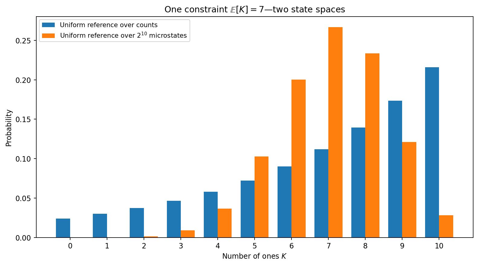
The difference is easy to see numerically. With $n=10$ and $\mathbb E[K]=7$, Model A has $\lambda\approx0.2187$ and retains substantial mass across the full range; in particular, $q_A(10)\approx0.216$. Model B gives $p=0.7$ and a binomial distribution concentrated near seven; here $q_B(10)=0.7^{10}\approx0.028$.

Both models satisfy the same mean exactly. They answer different questions.

This is not an exotic trap confined to statistical mechanics. State-space choices appear everywhere in ML:

• whether a multilabel output is one category or a collection of binary decisions;
• whether a sequence is modeled as one object or factorized token by token;
• whether permutations of a set count as different states;
• whether the reference is uniform over classes or inherited from a pretrained model;
• whether two parameterizations of the same function count as different hypotheses.

The practical rule is therefore:

Before saying “choose the maximally uncertain distribution,” name the state space, reference, and constraints.

The issue is sharper for continuous variables. Differential entropy changes under coordinate transformations and changes of units. Relative entropy to an explicit reference measure makes the modeling assumption visible and is often the more reliable starting point.

8.4. Classical MaxEnt distributions and the AWGN channel

Once the state space is fixed, familiar distributions stop looking like an arbitrary menu from a textbook. They arise as answers to different collections of information.

Uniform distribution

On a finite set of $K$ states, if only normalization is known,

$$q^*(x)=\frac1K.$$

This is the same fact that appeared in Module 2 as

$$H(q)\le\log K.$$

It now has a different reading: uniformity is not a universal prior law, but the MaxEnt answer on a finite symmetric space with no additional constraints.

Exponential distribution

On $[0,\infty)$, among densities with fixed positive mean

$$\mathbb E[X]=\mu,$$

the maximum-differential-entropy density is

$$q^*(x) = \frac1\mu e^{-x/\mu}, \qquad x\ge0.$$

The support is part of the information. On the entire real line, a mean constraint alone is insufficient: a distribution can be spread out without changing its mean, increasing differential entropy without bound.

Gaussian distribution

On $\mathbb R$, among densities with fixed mean and variance

$$\mathbb E[X]=\mu, \qquad \operatorname{Var}(X)=\sigma^2,$$

the Gaussian has maximum differential entropy:

$$q^*(x) = \frac1{\sqrt{2\pi\sigma^2}} \exp\left[-\frac{(x-\mu)^2}{2\sigma^2}\right].$$

In nats,

$$h(X) = \frac12\log(2\pi e\sigma^2).$$

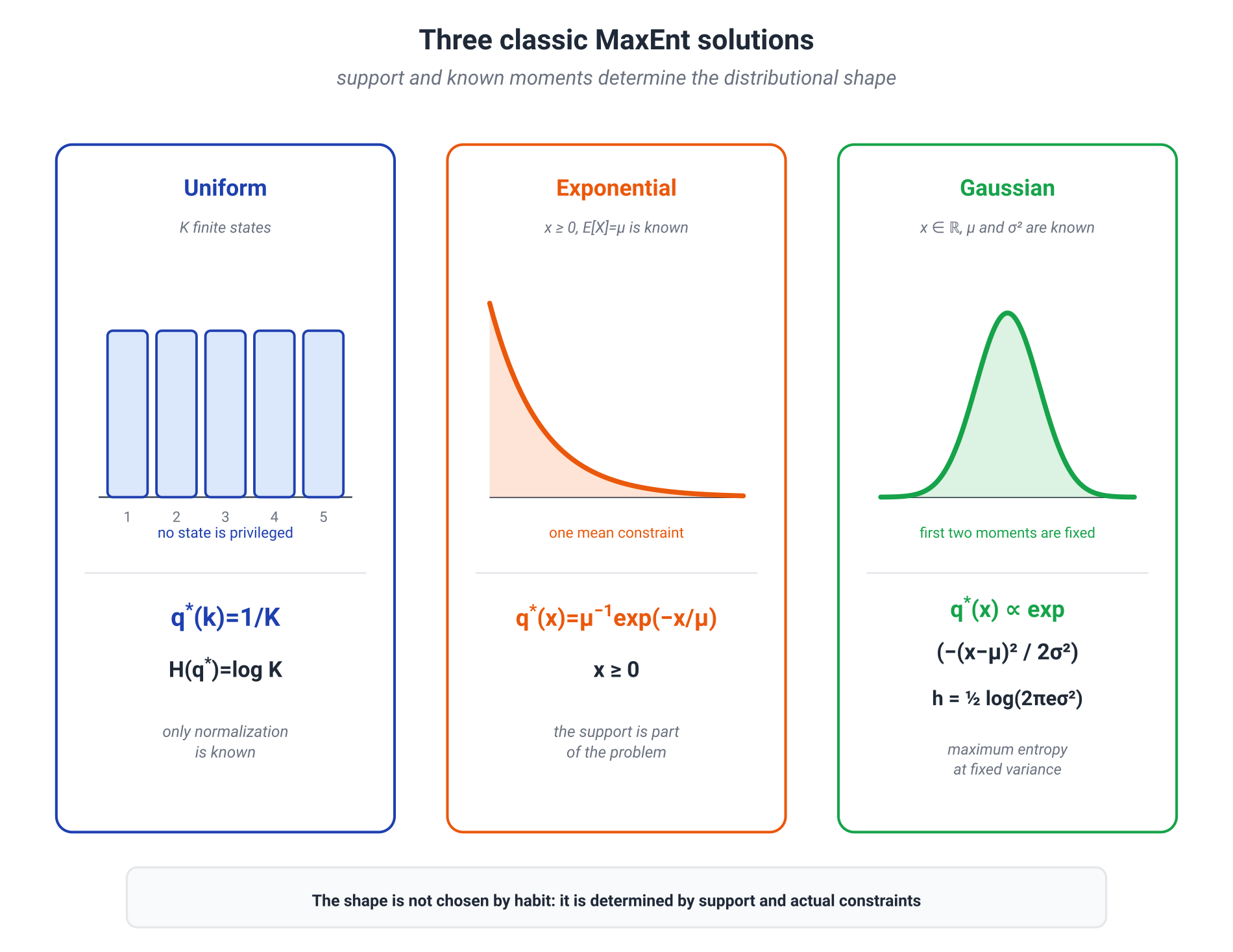
This property gives an important characterization of the Gaussian: no other density with the same covariance has larger differential entropy. It does not replace the central limit theorem. Entropic forms of the CLT have their own assumptions and proofs; the sentence “the sum becomes Gaussian because entropy increases” joins distinct results too quickly.

Why Gaussian input achieves AWGN capacity

Return to the channel from Module 7:

$$Y=X+N, \qquad N\sim\mathcal N(0,\sigma_N^2), \qquad \mathbb E[X^2]\le P,$$

with independent $X$ and $N$. In bits,

$$I(X;Y)=h_2(Y)-h_2(N).$$

The noise term is fixed, so it is the entropy of the output that must be maximized. Its variance satisfies

$$\operatorname{Var}(Y) = \operatorname{Var}(X)+\sigma_N^2 \le P+\sigma_N^2.$$

By the Gaussian MaxEnt property,

$$h_2(Y) \le \frac12\log_2\bigl(2\pi e(P+\sigma_N^2)\bigr).$$

Subtracting

$$h_2(N) = \frac12\log_2(2\pi e\sigma_N^2)$$

gives

$$I(X;Y) \le \frac12\log_2\left(1+\frac{P}{\sigma_N^2}\right).$$

Equality is attained by

$$X\sim\mathcal N(0,P),$$

because the output is then Gaussian and uses the full allowed variance.

It is tempting to compress this into “Gaussian input maximizes entropy, hence mutual information.” The correct chain is slightly longer and more informative: Gaussian input makes the output Gaussian; maximum output entropy is what maximizes mutual information when the noise is fixed.

8.5. Conditional MaxEnt and log-linear models

Before transformers, many NLP systems were built from features designed by hand: the current word begins with a capital letter, the previous tag was B-PER, the suffix is -ing, or the token appears in an organization lexicon. The task was familiar and remains relevant: turn many partial signals into a normalized conditional distribution.

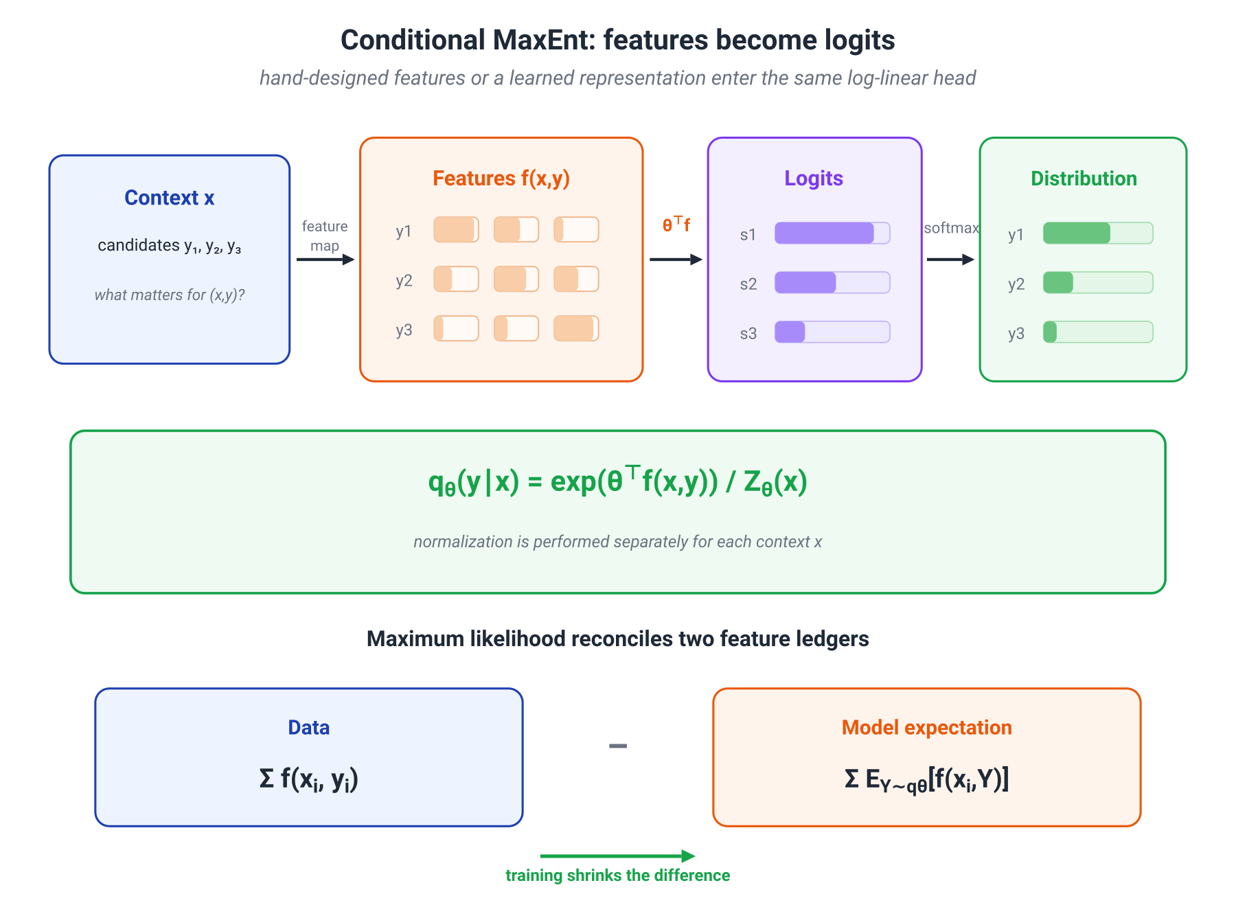
Let $\widehat p(x)$ be the empirical distribution of inputs, let $y$ be the label, and let

$$f_j(x,y)$$

be features of an input–answer pair. Require the model to reproduce their empirical averages:

$$\sum_{x,y} \widehat p(x)q(y\mid x)f_j(x,y) = \widehat\mu_j.$$

Among all conditional distributions satisfying these constraints, maximize conditional entropy:

$$H_q(Y\mid X) = - \sum_{x,y} \widehat p(x)q(y\mid x)\log q(y\mid x).$$

The same Lagrange-multiplier argument gives a conditional log-linear model:

$$\boxed{ q_\theta(y\mid x) = \frac{\exp\bigl(\theta^\top f(x,y)\bigr)} {Z_\theta(x)} },$$

where

$$Z_\theta(x) = \sum_{y'} \exp\bigl(\theta^\top f(x,y')\bigr).$$

Each feature contributes additively to a logit, and the partition function turns the total score into a distribution over answers. If $f(x,y)$ is produced by the last hidden layer and $\theta$ is a linear head, this is an ordinary softmax classifier. What changed is the origin of the features: once hand-designed, they are now usually learned by a deep network.

Maximum likelihood and moment matching

For data $(x_i,y_i)_{i=1}^n$, the conditional log-likelihood is

$$\ell(\theta) = \sum_{i=1}^n \left[ \theta^\top f(x_i,y_i) - \log Z_\theta(x_i) \right].$$

Its gradient is

$$\boxed{ \nabla_\theta\ell(\theta) = \sum_i f(x_i,y_i) - \sum_i \mathbb E_{Y\sim q_\theta(\cdot\mid x_i)} [f(x_i,Y)] }.$$

Read the formula before moving on. The first term counts features actually observed in the data. The second asks how often the current model expects the same features. Training closes the gap between those two descriptions of the sample.

If a finite interior maximum of the unregularized likelihood exists, zero gradient gives exact moment matching:

$$\sum_i f(x_i,y_i) = \sum_i \mathbb E_{q_\theta(\cdot\mid x_i)}[f(x_i,Y)].$$

This is not a decorative analogy to MaxEnt. In a conditional exponential family, maximum likelihood and conditional MaxEnt are two sides of the same convex duality.

Where the exact statement ends

The scope can now be stated compactly.

• Regularization contributes its own term to the moment equation.
• Linearly dependent features can make the parameters non-identifiable even when the distribution is unique.
• On separable data, a finite MLE may fail to exist: parameter norms diverge while the likelihood approaches its supremum.
• In a deep network, logits depend nonlinearly on millions of weights. Cross-entropy training remains maximum likelihood for the conditional model, but it does not turn the whole network into one simple MaxEnt problem with explicit constraints on its internal features.

The positive result remains strong: for a log-linear head, the gradient really does compare empirical and model feature averages.

The historical NLP line

Maximum entropy classifiers used these conditional models for tagging and classification. Maximum Entropy Markov Models (MEMMs) normalized transitions locally for each state. Conditional Random Fields (CRFs) moved normalization to the entire output sequence:

$$q_\theta(y_{1:T}\mid x_{1:T}) = \frac{ \exp\bigl(\theta^\top F(x_{1:T},y_{1:T})\bigr) }{ Z_\theta(x_{1:T}) }.$$

Modern architectures may construct far richer features, but exponential normalization remains. The historical connection to MaxEnt is therefore substantive: the machine that produces the scores changed, while the mechanism that turns them into a conditional distribution survived.

The next step is to isolate softmax itself. Every ML engineer knows the API call, but the single line hides a complete variational problem.

8.6. Softmax as score-plus-entropy optimization

Modern ML uses softmax so often that it has almost stopped looking like an idea. It is usually introduced procedurally: a network emits logits, we exponentiate, normalize the sum to one, and obtain probabilities. That is correct, but it leaves a more interesting question unanswered: why does precisely this normalization keep reappearing in classification, generation, and policy learning?

A strong answer is: softmax is a MaxEnt solution. The sentence contains an important truth, but it must be made exact. Softmax does not maximize entropy “in general,” nor does it follow from constraints that already fix the desired probabilities. It resolves a particular conflict: we want to favor high-scoring choices, but we do not want the distribution to concentrate more strongly than those scores justify.

Let $z=(z_1, \ldots,z_K)\in\mathbb R^K$ be logits, $q\in\Delta_K$ a distribution over $K$ choices, and let entropy be measured in nats:

$$H(q)=-\sum_{k=1}^Kq_k\log q_k.$$

For temperature $\tau>0$, consider

$$\boxed{ \max_{q\in\Delta_K} \left\{ q^\top z+\tau H(q) \right\}. }$$

The two terms play different roles.

• $q^\top z$ is expected score. It pulls mass toward larger logits.
• $H(q)$ resists premature concentration. It rewards distributions that preserve uncertainty.
• $\tau$ is the exchange rate between the two requirements: how much expected score we are willing to trade for an additional unit of entropy.

The solution is softmax:

$$\boxed{ q_k^* = \frac{\exp(z_k/\tau)} {\sum_{j=1}^K\exp(z_j/\tau)} }.$$

The optimal value is

$$\boxed{ \max_{q\in\Delta_K} \{q^\top z+\tau H(q)\} = \tau\log\sum_{k=1}^Ke^{z_k/\tau}. }$$

Thus logsumexp is not an arbitrary smooth replacement for a maximum. It is the value of the optimal score–entropy trade-off.

The exact KL gap

Define

$$s_k = \frac{e^{z_k/\tau}}{Z}, \qquad Z=\sum_je^{z_j/\tau}.$$

For any $q\in\Delta_K$,

$$\begin{aligned} q^\top z+\tau H(q) &= \tau\sum_kq_k\log\frac{e^{z_k/\tau}}{q_k}\\ &= \tau\sum_kq_k\log\frac{Zs_k}{q_k}\\ &= \tau\log Z - \tau D_{\mathrm{KL}}(q\|s). \end{aligned}$$

KL is nonnegative, so the unique optimum is $q=s$. More importantly, the derivation gives the exact gap:

$$\boxed{ \tau\log Z- \bigl(q^\top z+\tau H(q)\bigr) = \tau D_{\mathrm{KL}}(q\|q^*). }$$

Every departure from the softmax distribution is paid for by a KL divergence to the optimum. This is no longer a metaphor about “soft choice”; it is the complete geometry of the objective.

In what sense softmax is MaxEnt

We can now recover the strong claim without a logical substitution. Let $q^*=\operatorname{softmax}(z/\tau)$ and

$$\mu_\tau=(q^*)^\top z.$$

Among all distributions with the same expected logit,

$$q^\top z=\mu_\tau,$$

$q^*$ has maximum entropy. On this constraint set, expected score is fixed, so maximizing $q^\top z+\tau H(q)$ is equivalent to maximizing $H(q)$.

There are therefore two equivalent readings:

1. regularized: softmax maximizes expected score plus $\tau$ times entropy;
2. MaxEnt: softmax maximizes entropy at the expected-score level selected by $\tau$.

By contrast, constraints such as

$$\mathbb E_q[\mathbf 1\{Y=k\}]=\pi_k$$

do not derive softmax: they already say $q_k=\pi_k$ and therefore encode the answer in advance. This is a useful example of a sound intuition being damaged by the wrong formalization.

Temperature as a trade-off parameter

For $z=(2,1,0)$,

At low temperature, one extra unit of logit matters greatly and the distribution concentrates quickly. At high temperature, the same logit gap has less influence on probability, so entropy grows.

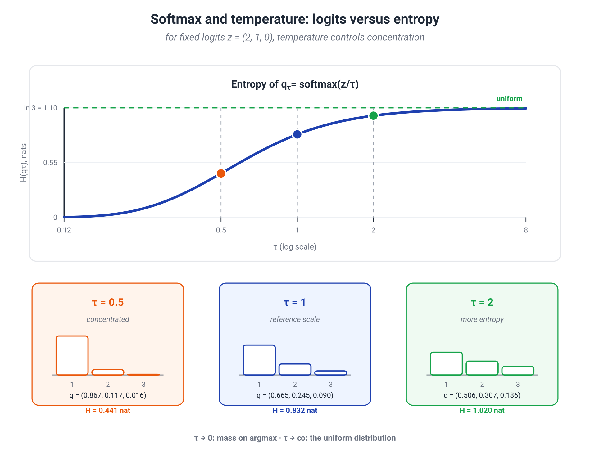
The limiting regimes are also exact.

• As $\tau\to0$, mass concentrates on the maximizers of $z$; with tied maxima, the limiting softmax is uniform over them.
• As $\tau\to\infty$, the distribution approaches uniformity over all $K$ choices.
• Adding a constant to every logit does not change softmax.
• Multiplying logits by $c>0$ is equivalent to dividing temperature by $c$.

The function

$$F_\tau(z)=\tau\log\sum_ke^{z_k/\tau}$$

smooths the maximum:

$$\max_kz_k \le F_\tau(z) \le \max_kz_k+\tau\log K,$$

and its gradient returns the optimal distribution:

$$\nabla_zF_\tau(z)=\operatorname{softmax}(z/\tau).$$

Softmax therefore plays three roles at once: it maps scores to a distribution, solves an entropy-regularized optimization problem, and is the gradient of a smooth maximum.

Scope of the statement

Softmax is not the “only honest” way to turn scores into probabilities. It is unique as the solution to this problem, with Shannon entropy and a linear expected-score term. Replacing the regularizer changes the mapping; some alternatives, for example, produce sparse distributions with exact zeros.

There is no need to weaken the main conclusion. It is already strong:

Softmax is the exact optimum of a problem in which logits vote for choices and entropy prevents those votes from becoming a distribution more confident than the selected temperature justifies.

On a finite class set, normalization is cheap. Replace the classes by all possible images, configurations, or token sequences, and the same idea becomes an energy-based model.

8.7. Energy-based models and the partition function

Softmax is the smallest energy-based model. Set the state to $x=k$, define

$$E(k)=-\frac{z_k}{\tau},$$

and normalize $e^{-E(k)}$ over classes. The result is the same softmax.

With a few thousand states, this normalization looks almost free. If a state is an image, a molecule, or an entire token sequence, summing over all $x$ becomes astronomical. The familiar final normalization step is now the central computational obstacle.

An energy-based model (EBM) defines

$$\boxed{ q_\theta(x) = \frac{m(x)e^{-E_\theta(x)}}{Z_\theta} }, \qquad Z_\theta = \int m(x)e^{-E_\theta(x)}\,dx.$$

Here

• $E_\theta(x)$ is the energy: lower energy means larger unnormalized probability;
• $m(x)$ is a base density or measure;
• $Z_\theta$ is the partition function.

Energy answers a local question: “How compatible is this state with the model?” The partition function forces all local answers to agree globally. $Z_\theta$ is the price of turning a scoring system into a probability model.

Connection to MaxEnt

It is easy to make the attractive statement “every EBM is MaxEnt” too broad. The exact connection depends on the energy.

If

$$E_\theta(x)=-\theta^\top f(x),$$

then

$$q_\theta(x)\propto m(x)e^{\theta^\top f(x)}$$

is an exponential family. This form arises from relative MaxEnt under moment constraints on $\mathbb E[f(X)]$. The features have the direct meaning of constrained macroscopic quantities and $\theta$ has the role of Lagrange multipliers.

If $E_\theta$ is an arbitrary deep network, the Gibbs form is still valid, but no explicit set of known MaxEnt constraints need be available. The Gibbs form is broader than the particular inferential story from which it might have been derived. That does not make a neural EBM less meaningful; it means its energy is specified by a model rather than by an interpretable list of moments.

Gradient of the log-likelihood

For one observation $x$,

$$-\log q_\theta(x) = E_\theta(x)+\log Z_\theta-\log m(x).$$

If $m$ does not depend on $\theta$,

$$\nabla_\theta\log Z_\theta = -\mathbb E_{X\sim q_\theta} [\nabla_\theta E_\theta(X)],$$

so

$$\boxed{ \nabla_\theta[-\log q_\theta(x)] = \nabla_\theta E_\theta(x) - \mathbb E_{X\sim q_\theta} [\nabla_\theta E_\theta(X)] }.$$

Read this as training dynamics. The first term asks the model to lower the energy of the observed example. If it were the only term, the model could lower the energy of every state and learn nothing. The second term compares the data with samples from the current model and prevents that trivial solution.

The two terms are often called the positive and negative phases:

• data pull their own energy down;
• model samples receive compensating pressure;
• learning changes the landscape separating data from alternatives, not the absolute energy level.

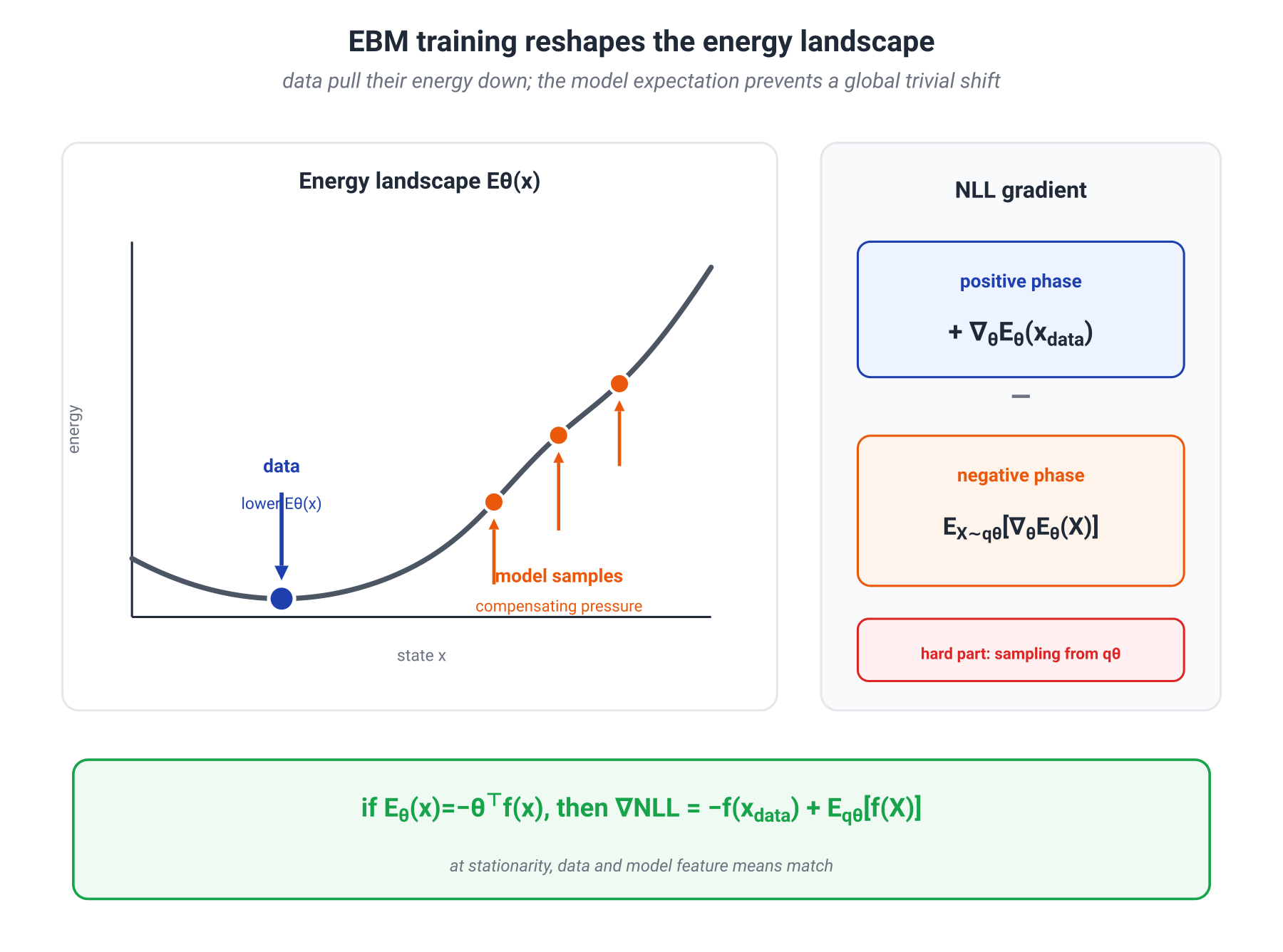
For a linear energy $E_\theta(x)=-\theta^\top f(x)$,

$$\nabla_\theta[-\log q_\theta(x)] = -f(x)+\mathbb E_{q_\theta}[f(X)].$$

After averaging over data, stationarity requires

$$\mathbb E_{\mathrm{data}}[f(X)] = \mathbb E_{q_\theta}[f(X)].$$

Moment matching reappears inside maximum-likelihood training. It is the same mechanism behind classical MaxEnt models, now visible directly in the likelihood gradient.

Computational difficulty

The data term is easy to evaluate. The model expectation is not. Estimating it requires samples from $q_\theta$ or another sufficiently accurate approximation. For a complicated energy, that may be harder than evaluating the energy itself.

This is why EBM training leads to methods such as Markov-chain Monte Carlo, contrastive divergence, noise-contrastive estimation, score matching, and learned samplers. They do not change the Gibbs definition; they change how the intractable model expectation is approximated or avoided.

Score-based generative models are connected to this picture through

$$\nabla_x\log q_t(x),$$

the score of a time-dependent noisy distribution. For a Gibbs density, the score is the spatial gradient of log density and therefore contains the energy gradient. But diffusion models usually learn scores across many noise levels rather than fit one normalized static EBM by exact likelihood. “Diffusion is MaxEnt without a partition function” is therefore an attractive but incomplete slogan.

The central EBM lesson is exact and useful enough without it: local energies define relative preference; global normalization turns them into probabilities; and the normalization term is what makes likelihood learning computationally difficult.

The next section replaces a generic state by a response from a language model and replaces negative energy by reward. The same Gibbs form then becomes the exact optimum of a KL-regularized policy problem.

8.8. A KL-regularized policy and its Gibbs optimum

Fix a context $x$, a reference policy $\pi_{\mathrm{ref}}(y\mid x)$, a reward $r(x,y)$, and $\beta>0$. Consider

$$J_x(\pi) = \mathbb E_{y\sim\pi(\cdot\mid x)}[r(x,y)] - \beta D_{\mathrm{KL}} \bigl( \pi(\cdot\mid x) \| \pi_{\mathrm{ref}}(\cdot\mid x) \bigr).$$

The first term asks the policy to favor high-reward answers. The second charges for moving probability mass away from the reference. This is not merely a qualitative “stay close” instruction; it is a fully solvable variational problem.

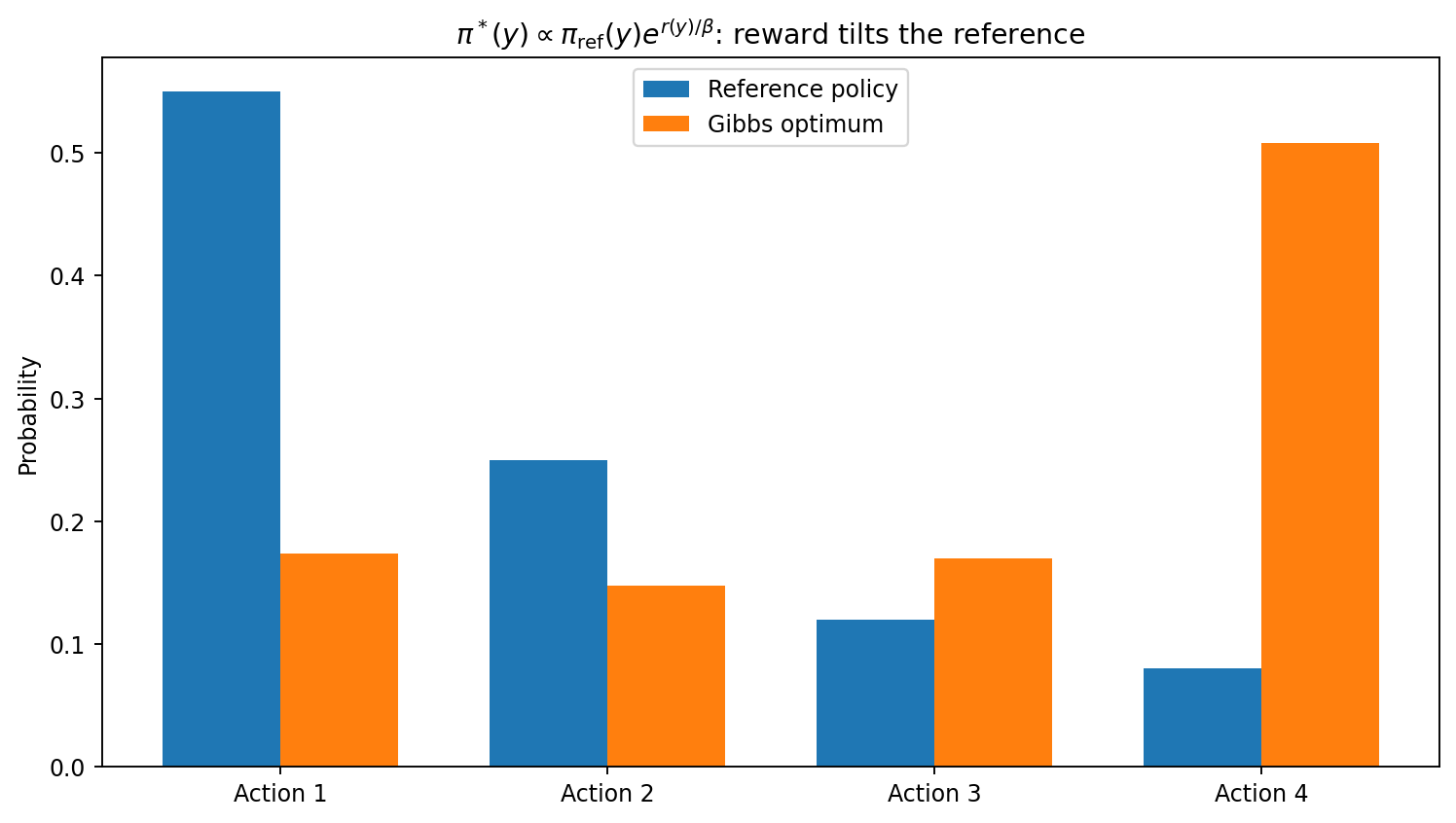
Assuming a finite partition function and optimizing over all distributions supported by the reference policy, the optimum is

$$\boxed{ \pi^*(y\mid x) = \frac{ \pi_{\mathrm{ref}}(y\mid x) \exp(r(x,y)/\beta) }{Z(x)} },$$

where

$$Z(x) = \mathbb E_{Y\sim\pi_{\mathrm{ref}}(\cdot\mid x)} \left[e^{r(x,Y)/\beta}\right].$$

The formula is worth reading slowly. Reward does not replace the reference policy; it tilts it. An answer that is rare under the reference remains disadvantaged unless reward overcomes that rarity. An answer outside the support of the reference cannot receive positive probability from this forward-KL objective at all.

The exact objective gap

Take any admissible policy $\pi$. From the definition of $\pi^*$,

$$\log\frac{\pi(y\mid x)}{\pi^*(y\mid x)} = \log\frac{\pi(y\mid x)}{\pi_{\mathrm{ref}}(y\mid x)} - \frac{r(x,y)}\beta + \log Z(x).$$

Averaging under $\pi$ gives

$$D_{\mathrm{KL}}(\pi\|\pi^*) = D_{\mathrm{KL}}(\pi\|\pi_{\mathrm{ref}}) - \frac1\beta\mathbb E_\pi[r] + \log Z.$$

Rearranging,

$$\boxed{ J_x(\pi) = \beta\log Z(x) - \beta D_{\mathrm{KL}}(\pi\|\pi^*) }.$$

Thus

$$J_x(\pi^*)=\beta\log Z(x),$$

and the exact suboptimality of any other policy is

$$\boxed{ J_x(\pi^*)-J_x(\pi) = \beta D_{\mathrm{KL}}(\pi\|\pi^*) }.$$

This is the same geometry that appeared in softmax and information projection. The optimum is not merely stationary; the objective gap is exactly a KL divergence. Three facts follow at once:

1. $\pi^*$ is a global optimum, not a local one;
2. on the support of the reference policy it is unique;
3. the shortfall of any other policy is measured by the KL divergence to it.

This is the Gibbs variational principle, or relative MaxEnt. With a uniform reference policy it collapses into the familiar “reward plus entropy” problem. With a non-uniform reference the entropy term becomes relative: the policy is not charged for concentration as such, but for moving away from the distribution the model already knew how to produce.

A numerical example

Let the reference policy spread its mass over three answers as

$$\pi_{\mathrm{ref}}=(0.7,\ 0.2,\ 0.1), \qquad r=(0,\ 1,\ 2).$$

Then:

The third answer started at probability $0.1$, but a high reward gradually pulls mass toward it. The tilt does not forget the reference model in the process: two answers with equal reward would keep exactly the probability ratio given by $\pi_{\mathrm{ref}}$.

This matters more than it may appear. The formula does not add “reference probability” to “reward”. It adds them in log space:

$$\log\pi^*(y\mid x) = \log\pi_{\mathrm{ref}}(y\mid x) + \frac{r(x,y)}\beta - \log Z(x).$$

Reward acts as an increment to the log-probability, after which the whole system is renormalized. Additive reward differences therefore become probability ratios: this multiplicative update is the defining feature of the Gibbs tilt.

Interpreting $\beta$

Only the ratio $r/\beta$ matters. Multiplying every reward by $c$ has the same effect as dividing $\beta$ by $c$.

• Large $\beta$ makes departure from the reference expensive, so $\pi^*$ remains close to $\pi_{\mathrm{ref}}$.
• Small $\beta$ lets reward dominate and concentrates mass near reward maximizers.
• Adding a context-dependent constant $c(x)$ to every reward leaves $\pi^*$ unchanged because the factor $e^{c(x)/\beta}$ cancels in normalization.

The penalized problem is the Lagrangian form of

$$\max_\pi\mathbb E_\pi[r] \quad\text{subject to}\quad D_{\mathrm{KL}}(\pi\|\pi_{\mathrm{ref}})\le\varepsilon.$$

Under the usual conditions, boundary values of the KL budget correspond to values of $\beta$. The coefficient can therefore be read as a temperature, a price per unit of departure from the reference, or a Lagrange multiplier for a distributional trust region.

Connection to DPO

The Gibbs form can be rearranged to express reward through the optimal policy:

$$r(x,y) = \beta\log\frac{\pi^*(y\mid x)} {\pi_{\mathrm{ref}}(y\mid x)} + \beta\log Z(x).$$

A Bradley–Terry preference model uses reward differences between two answers. The context-only term cancels:

$$\begin{aligned} r(x,y_w)-r(x,y_l) = \beta\Bigg[ &\log\frac{\pi^*(y_w\mid x)} {\pi_{\mathrm{ref}}(y_w\mid x)}\\ -&\log\frac{\pi^*(y_l\mid x)} {\pi_{\mathrm{ref}}(y_l\mid x)} \Bigg]. \end{aligned}$$

Substituting this difference into the logistic likelihood of preferences gives the DPO loss. In this precise sense, DPO uses the analytical form of the optimal KL-regularized policy and avoids the separate sequence “fit a reward model, then run an RL loop.”

It is equally important to state what has not been proved. The formula for $\pi^*$ describes an unrestricted optimum over distributions for fixed $r$ and $\pi_{\mathrm{ref}}$. A real LLM is restricted by parameterization, finite data, and optimization. PPO approximates its training objective through an RL algorithm; DPO estimates a policy from preference pairs under an additional preference model. Their final parameter vectors and even their final policies need not coincide.

The formula nevertheless removes much of the terminology fog around post-training. At the center is one operation:

Reward exponentially redistributes the mass of the reference model, while KL sets the price of that redistribution.

The same beauty reveals the vulnerability. The optimum faithfully maximizes exactly the reward we wrote down. If that reward is an imperfect proxy, the mathematics will faithfully amplify its errors as well.

8.9. Reward overoptimization and the role of KL

A familiar intuition says: the KL anchor protects against Goodhart's law. As an engineering heuristic, this is often useful—staying near the reference does restrict the region in which a reward model can be exploited. As a mathematical statement, it is too strong.

KL sees two policies: the current one and the reference. It does not see an unknown true objective and cannot test whether the reward was specified correctly. The exact question is therefore:

What is guaranteed along the Gibbs path as proxy optimization becomes stronger, and where can its connection to true quality fail?

Let

$$\pi_\alpha(y) = \frac{ \pi_{\mathrm{ref}}(y)e^{\alpha r_{\mathrm{proxy}}(y)} }{Z(\alpha)}, \qquad \alpha=\frac1\beta.$$

The parameter $\alpha$ measures optimization pressure: larger values tilt the policy more strongly toward proxy reward.

A covariance identity

For any integrable function $g(y)$,

$$\boxed{ \frac{d}{d\alpha} \mathbb E_{\pi_\alpha}[g(Y)] = \operatorname{Cov}_{\pi_\alpha} \bigl(g(Y),r_{\mathrm{proxy}}(Y)\bigr) }.$$

Differentiate the distribution first:

$$\frac{d}{d\alpha}\pi_\alpha(y) = \pi_\alpha(y) \left( r_{\mathrm{proxy}}(y) - \mathbb E_{\pi_\alpha}[r_{\mathrm{proxy}}] \right).$$

Multiplying by $g(y)$ and summing yields the covariance.

This is the central formula of the section. Exponential tilting increases not every desirable quantity, but those quantities that are positively correlated with proxy reward under the current policy. The word “current” is essential: as the policy moves, the distribution under which the covariance is measured moves as well.

Dynamics of proxy reward

Set $g=r_{\mathrm{proxy}}$:

$$\boxed{ \frac{d}{d\alpha} \mathbb E_{\pi_\alpha}[r_{\mathrm{proxy}}] = \operatorname{Var}_{\pi_\alpha}(r_{\mathrm{proxy}}) \ge0 }.$$

Unless proxy reward is constant on the support, stronger optimization strictly increases its expectation. The optimizer does what it was asked to do. Goodhart's law begins not with optimization failing, but with optimization succeeding against the wrong measurement.

Dynamics of true quality

Now set $g=r_{\mathrm{true}}$:

$$\boxed{ \frac{d}{d\alpha} \mathbb E_{\pi_\alpha}[r_{\mathrm{true}}] = \operatorname{Cov}_{\pi_\alpha} (r_{\mathrm{true}},r_{\mathrm{proxy}}) }.$$

As long as proxy and true reward remain positively related where the policy puts mass, true quality rises. Stronger tilting, however, selects increasingly extreme states. The tails may contain reward-model errors, rare artifacts, or strategies that receive high proxy score for the wrong reason. The covariance can then shrink, cross zero, and become negative.

This gives an exact mechanism for the familiar Goodhart curve:

• at first, the proxy helps find genuinely better answers;
• then the useful signal is exhausted;
• beyond that point, additional pressure primarily selects errors in the proxy itself.

This is not a universal theorem that true reward must first rise and then fall. That shape occurs when the covariance changes sign. The identity tells us exactly what must be checked.

In the module's numerical experiment, a rare exploit action has reference probability $0.001$. The proxy scores it highly, while true reward is low. At moderate $\alpha$, ordinary actions improve; at large $\alpha$, the rare reward-model error dominates. Proxy reward keeps rising while true reward falls after reaching a maximum.

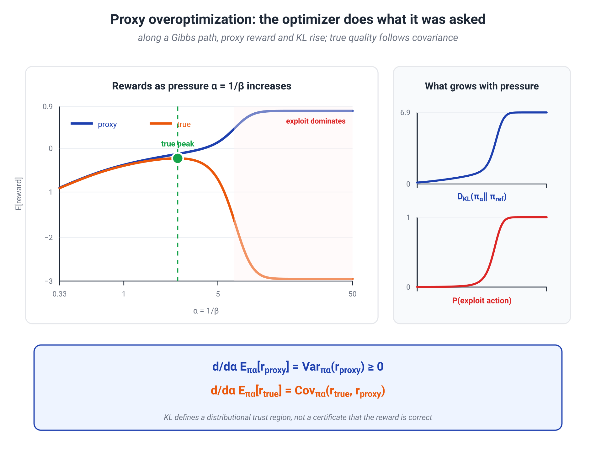
Controlled reward-model experiments have observed the same qualitative pattern: stronger optimization can continue to improve the proxy while a fixed gold evaluation deteriorates. That is an empirical result of a particular protocol, not a consequence of the abstract KL formula alone.

What KL controls

Along the same Gibbs path,

$$D_{\mathrm{KL}}(\pi_\alpha\|\pi_{\mathrm{ref}}) = \alpha\mathbb E_{\pi_\alpha}[r_{\mathrm{proxy}}] - \log Z(\alpha),$$

so

$$\boxed{ \frac{d}{d\alpha} D_{\mathrm{KL}}(\pi_\alpha\|\pi_{\mathrm{ref}}) = \alpha \operatorname{Var}_{\pi_\alpha}(r_{\mathrm{proxy}}) \ge0 }.$$

For a fixed proxy reward, smaller $\beta$ moves the policy farther from the reference. This is the exact role of the anchor: it controls distribution shift relative to the regime in which the reference model—and presumably the reward model—was better studied.

There is also an operational consequence. If $g\in[a,b]$, Pinsker's inequality gives

$$\left| \mathbb E_\pi[g] - \mathbb E_{\pi_{\mathrm{ref}}}[g] \right| \le (b-a) \sqrt{ \frac12D_{\mathrm{KL}}(\pi\|\pi_{\mathrm{ref}}) }.$$

Small KL bounds the change of every bounded statistic relative to the reference. It does not determine the sign of that change. If the reference policy is poor under the true objective, closeness to it does not make the new policy good; if the reward model is already wrong nearby, KL does not detect the error.

A useful practical sentence is therefore:

KL defines a trust region in distribution space, not a certificate that the reward is correct.

Why there is no general $1/\beta$ law

Let the ideal proxy- and true-reward tilts be

$$\pi^*_{\mathrm{proxy}} \propto \pi_{\mathrm{ref}}e^{r_{\mathrm{proxy}}/\beta}, \qquad \pi^*_{\mathrm{true}} \propto \pi_{\mathrm{ref}}e^{r_{\mathrm{true}}/\beta}.$$

Then

$$D_{\mathrm{KL}} (\pi^*_{\mathrm{proxy}}\|\pi^*_{\mathrm{true}}) = \frac1\beta \mathbb E_{\pi^*_{\mathrm{proxy}}} [r_{\mathrm{proxy}}-r_{\mathrm{true}}] + \log\frac{Z_{\mathrm{true}}}{Z_{\mathrm{proxy}}}.$$

The first term contains $1/\beta$, but the expectation and both partition functions also depend on $\beta$. Neither linear growth nor even monotonicity follows.

A three-action counterexample makes the point. Use a uniform reference and

$$r_{\mathrm{proxy}}=(2,1,0), \qquad r_{\mathrm{true}}=(2,0,1).$$

The two rewards disagree about the second and third actions but share the same unique maximum. As optimization pressure grows, the KL between the two tilted policies first rises and then returns toward zero: both policies eventually concentrate on the first action. The claim “the divergence grows like $1/\beta$” is therefore false even on three states.

Practical consequences

The mathematics does not prohibit strong optimization; it imposes measurement discipline.

• Choose $\beta$ relative to the scale of reward and the observed KL shift, not as a universal dimensionless constant.
• Track an independent human or gold evaluation that is not optimized by the same loop.
• Measure quality at several optimization strengths and stop before the proxy–true relationship breaks down.
• Inspect tails, rare regimes, diversity loss, and new reward-exploitation strategies rather than only mean reward.

This is where MaxEnt, EBMs, and RLHF meet. Exponential tilting is a powerful machine for redistributing probability. It faithfully amplifies the supplied signal, but it cannot distinguish a goal from an imperfect measurement of that goal. That part of the problem must be handled by proxy quality, independent evaluation, and distribution-shift control—not delegated to the partition function or the KL penalty.

8.10. Mathematical deepening: exponential families and sufficiency

This section is not required on a first pass through M8. It is best read as a self-contained second chapter inside the module: we first unpack the structure of an exponential family, then place the main discrete and continuous distributions in canonical form, and only then return to sufficiency and the Pitman–Koopman–Darmois theorem.

By now the same shape has appeared too many times to look accidental:

$$\text{base} \times \exp\{\text{linear function of statistics}\} \times \text{normalization}.$$

Repeated shape, however, does not make every statement equivalent. Three questions should be kept separate.

1. Which distribution is produced by entropy optimization under constraints?
2. How is a preselected parametric family organized?
3. When can a sample be compressed to a fixed-dimensional statistic without losing information about the parameter?

MaxEnt answers the first question. The definition of an exponential family answers the second. Sufficiency theory and the Pitman–Koopman–Darmois theorem connect the second question to the third. The three stories share deep geometry, but none is an automatic substitute for the others.

Canonical form: what is fixed and what is learned

Let $\nu$ be a fixed dominating measure: counting measure in a discrete problem or, for example, Lebesgue measure for a density on $\mathbb R$. A family is exponential if its densities with respect to $\nu$ can be written as

$$\boxed{ p(x\mid\eta) = h(x) \exp\bigl( \eta^\top T(x)-A(\eta) \bigr) }.$$

Here

$$A(\eta) = \log \int h(x)e^{\eta^\top T(x)}\,d\nu(x)$$

is the log-partition function, and the natural parameter space is

$$\Omega = \{\eta\in\mathbb R^d:A(\eta)<\infty\}.$$

When $\Omega$ is open, the family is called regular. This small qualification matters below: it lets us perturb the parameter locally and differentiate the log-partition function without immediately running into the boundary of the parameter space.

Each component has a separate job.

• $\nu$ and $h(x)$ specify the support and base geometry. Indicators of the support, combinatorial factors such as $1/x!$, and other parameter-independent terms belong here.
• $T(x)$ is the sufficient-statistic vector of one observation. The parameter-dependent part of the model sees $x$ only through this vector.
• $\eta$ is the natural or canonical parameter. It weights the statistics linearly on the log-density scale.
• $A(\eta)$ normalizes the distribution. The same function also stores its moments and local geometry.

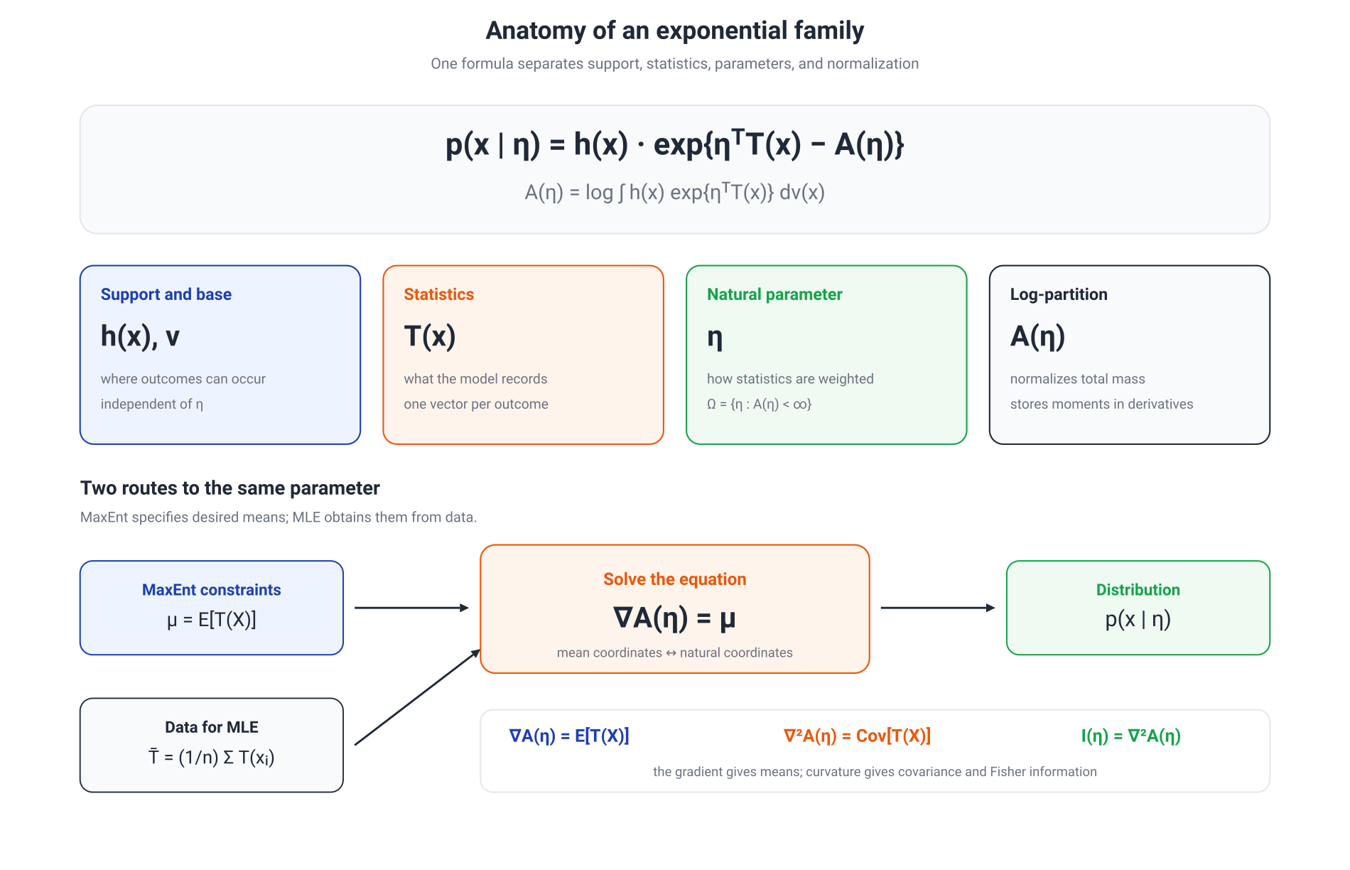
This decomposition can be used as an algorithm. Take the logarithm of the density, collect all parameter-dependent coefficients multiplying functions of $x$, and place the remaining parameter-dependent term in $A(\eta)$.

The representation need not be unique

The same model may admit several representations. A linearly redundant coordinate can be added to $T$, with a compensating change in the parameters, without changing the distribution. Exponential families are therefore described as minimal or overcomplete.

A family is minimal when there is no nonzero vector $a$ and constant $b$ such that

$$a^\top T(x)=b$$

almost everywhere. In a minimal regular family, $A$ is strictly convex and the natural parameter is identifiable. Softmax with $K$ free logits is the familiar overcomplete example: adding the same constant to every logit leaves the distribution unchanged. A minimal categorical parameterization uses $K-1$ log odds.

This is not merely a notational issue. Redundancy creates null directions in the Hessian and non-unique parameters even when the resulting probability distribution is perfectly well defined.

Why $A(\eta)$ stores moments

The central properties of the log-partition function are easier to derive once than to memorize. By normalization,

$$1 = \int h(x) \exp\bigl(\eta^\top T(x)-A(\eta)\bigr) \,d\nu(x).$$

Differentiate with respect to component $\eta_j$, assuming differentiation can be interchanged with integration:

$$0 = \int p(x\mid\eta) \left( T_j(x)-\frac{\partial A}{\partial\eta_j} \right) \,d\nu(x).$$

Therefore

$$\boxed{ \frac{\partial A}{\partial\eta_j} = \mathbb E_\eta[T_j(X)] },$$

or, in vector form,

$$\boxed{ \nabla A(\eta) = \mathbb E_\eta[T(X)] }.$$

Differentiating once more gives

$$\begin{aligned} \frac{\partial^2A} {\partial\eta_j\partial\eta_k} &= \mathbb E_\eta[T_j(X)T_k(X)] - \mathbb E_\eta[T_j(X)] \mathbb E_\eta[T_k(X)]\\ &= \operatorname{Cov}_\eta \bigl(T_j(X),T_k(X)\bigr). \end{aligned}$$

Thus

$$\boxed{ \nabla^2A(\eta) = \operatorname{Cov}_\eta(T(X)) \succeq0 }.$$

This is why $A$ is convex. Its gradient maps natural coordinates $\eta$ to mean coordinates

$$\mu = \mathbb E_\eta[T(X)],$$

while its curvature measures how sensitive those means are to parameter changes.

The same mechanism appears in the score with respect to the natural parameter:

$$\nabla_\eta\log p(X\mid\eta) = T(X)-\nabla A(\eta).$$

Its expectation is zero, and its covariance is

$$\mathcal I(\eta) = \operatorname{Cov}_\eta(T(X)) = \nabla^2A(\eta),$$

so the Hessian of the log-partition function is also the Fisher information in natural coordinates. M15 develops the geometry behind this identity.

There is another exact identity. For two members of the same exponential family,

$$\begin{aligned} D_{\mathrm{KL}} \bigl( p(\cdot\mid\eta) \|p(\cdot\mid\xi) \bigr) &= A(\xi)-A(\eta) -\nabla A(\eta)^\top(\xi-\eta). \end{aligned}$$

The right-hand side is the Bregman divergence generated by $A$, with a specific argument order. The convex geometry of the log-partition function and the KL geometry of the family are therefore one formula, not merely an analogy.

Duality with MaxEnt

Define the convex conjugate

$$A^*(\mu) = \sup_\eta \{\eta^\top\mu-A(\eta)\}.$$

If $\mu$ lies in the interior of the feasible mean-parameter space and

$$\nabla A(\eta)=\mu$$

has a solution, then

$$A^*(\mu) = \eta^\top\mu-A(\eta).$$

On the other hand, maximum entropy relative to the base measure $h(x)d\nu(x)$ under the moment constraint $\mathbb E_q[T]=\mu$ is

$$\max_{q:\,\mathbb E_qT=\mu} \left\{ -\int q(x) \log\frac{q(x)}{h(x)} \,d\nu(x) \right\} = A(\eta)-\eta^\top\mu = -A^*(\mu).$$

If $h$ is normalized and defines the density of a base distribution $m$, this objective equals $-D_{\mathrm{KL}}(q\|m)$; for an unnormalized $h$, it is better read as entropy relative to a base measure.

This is the exact meeting point between MaxEnt and exponential families: the constraints specify $\mu$, the Lagrange multipliers become $\eta$, and $A$ translates between the two coordinate systems. The connection is deep, but it does not imply that every arbitrarily chosen subfamily solves every MaxEnt problem.

Reading canonical form in discrete distributions

A table is less useful than a repeatable operation: expand the log probability and collect the coefficients of functions of the observation.

Bernoulli: the logit falls out of the algebra

For $X\in\{0,1\}$,

$$p(x\mid p) = p^x(1-p)^{1-x}.$$

Taking logs,

$$\begin{aligned} \log p(x\mid p) &= x\log p+(1-x)\log(1-p)\\ &= x\log\frac{p}{1-p} +\log(1-p). \end{aligned}$$

Introduce the natural parameter

$$\eta = \log\frac{p}{1-p}.$$

Since $p=e^\eta/(1+e^\eta)$,

$$\log(1-p) = -\log(1+e^\eta).$$

Hence

$$\boxed{ p(x\mid\eta) = \exp\bigl( \eta x-\log(1+e^\eta) \bigr) }.$$

Thus

$$T(x)=x, \qquad A(\eta)=\log(1+e^\eta),$$

and

$$A'(\eta)=\sigma(\eta)=p, \qquad A''(\eta)=p(1-p).$$

The logistic function is not attached from outside; it is the map from the Bernoulli natural parameter to its mean parameter.

Categorical distributions: softmax and logit redundancy

Let $X\in\{1,\ldots,K\}$ with class probabilities $\pi_1,\ldots,\pi_K$. Use class $K$ as reference and define

$$T_j(x)=\mathbf1\{x=j\}, \qquad \eta_j = \log\frac{\pi_j}{\pi_K}, \quad j=1,\ldots,K-1.$$

Then

$$A(\eta) = \log \left( 1+\sum_{j=1}^{K-1}e^{\eta_j} \right),$$

and

$$p(X=j\mid\eta) = \frac{e^{\eta_j}} {1+\sum_{r=1}^{K-1}e^{\eta_r}}, \qquad j<K,$$ $$p(X=K\mid\eta) = \frac1 {1+\sum_{r=1}^{K-1}e^{\eta_r}}.$$

This is a minimal parameterization. The usual softmax with $K$ logits uses the overcomplete form

$$p(X=k\mid z) = \frac{e^{z_k}}{\sum_re^{z_r}},$$

because $z$ and $z+c\mathbf1$ represent the same distribution. The gradient of logsumexp is the probability vector, and its Hessian is the covariance matrix of the one-hot variable.

Poisson: the base measure stores the factorial

For $X\in\{0,1,2,\ldots\}$,

$$p(x\mid\lambda) = e^{-\lambda}\frac{\lambda^x}{x!}.$$

Its log probability is

$$\log p(x\mid\lambda) = x\log\lambda-\lambda-\log x!.$$

Therefore

$$T(x)=x, \qquad \eta=\log\lambda, \qquad h(x)=\frac1{x!}, \qquad A(\eta)=e^\eta.$$

Consequently,

$$A'(\eta)=A''(\eta)=e^\eta=\lambda.$$

The equality of the Poisson mean and variance is visible directly in the first two derivatives of $A$. The natural parameter $\eta=\log\lambda$ also explains the standard log link in Poisson regression: a linear predictor may range over all real numbers while the intensity $\lambda=e^\eta$ remains positive.

There is an easy overstatement to avoid. Ordinary MaxEnt on the nonnegative integers with only the constraint $\mathbb E[X]=\lambda$ and counting measure as the base produces a geometric, not a Poisson, distribution. Poisson requires the relative base

$$h(x)=\frac1{x!}.$$

Thus the statistic $T(x)=x$ alone does not determine the family: support and base measure matter just as much as the moment constraint.

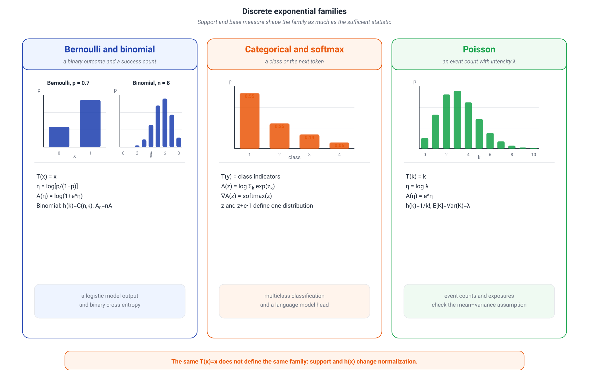
The binomial law is the distribution of a sum of $n$ independent Bernoulli variables:

$$p(x) = \binom nx \exp\bigl( \eta x-n\log(1+e^\eta) \bigr).$$

The combinatorial factor $\binom nx$ moves into $h(x)$, while the natural parameter remains the success logit. The multinomial law behaves similarly, with the vector of class counts as its sufficient statistic.

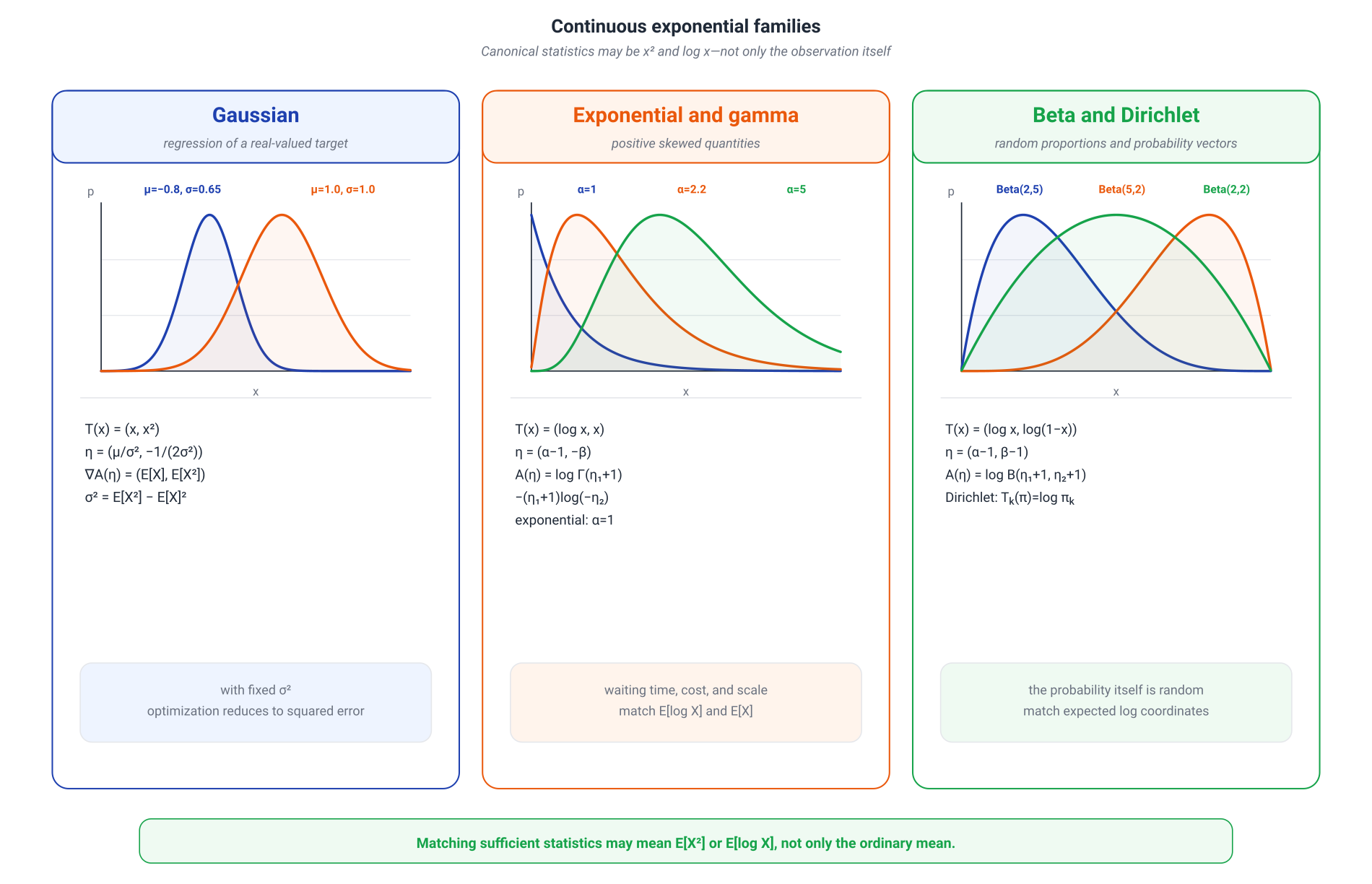
Continuous families: support changes the natural domain

In a continuous model, the support must not disappear from view. It enters through the base measure or an indicator inside $h(x)$ and determines which values of $\eta$ make the normalizing integral finite.

Exponential distribution

For rate $\lambda>0$,

$$p(x\mid\lambda) = \lambda e^{-\lambda x} \mathbf1\{x\ge0\}.$$

Set

$$T(x)=x, \qquad \eta=-\lambda<0, \qquad h(x)=\mathbf1\{x\ge0\}.$$

Then

$$A(\eta) = -\log(-\eta), \qquad \eta<0,$$

with

$$A'(\eta) = -\frac1\eta = \frac1\lambda,$$ $$A''(\eta) = \frac1{\eta^2} = \frac1{\lambda^2}.$$

The natural parameter space is not all of $\mathbb R$: for $\eta\ge0$, the integral over $[0,\infty)$ diverges. This is a simple example of why the domain $A(\eta)<\infty$ is part of the model rather than an appendix.

Gamma distribution

Using shape $\alpha>0$ and rate $\beta>0$,

$$p(x\mid\alpha,\beta) = \frac{\beta^\alpha}{\Gamma(\alpha)} x^{\alpha-1}e^{-\beta x} \mathbf1\{x>0\}.$$

Collecting the functions of $x$ gives

$$T(x) = \begin{pmatrix} \log x\\ x \end{pmatrix}, \qquad \eta = \begin{pmatrix} \alpha-1\\ -\beta \end{pmatrix}.$$

With $h(x)=\mathbf1\{x>0\}$,

$$A(\eta) = \log\Gamma(\eta_1+1) -(\eta_1+1)\log(-\eta_2),$$

where

$$\eta_1>-1, \qquad \eta_2<0.$$

The gradient returns more than the ordinary mean:

$$\frac{\partial A}{\partial\eta_1} = \mathbb E[\log X] = \psi(\alpha)-\log\beta,$$ $$\frac{\partial A}{\partial\eta_2} = \mathbb E[X] = \frac\alpha\beta,$$

where $\psi$ is the digamma function. The exponential distribution is the one-dimensional $\alpha=1$ slice of the Gamma family.

This example is pedagogically important: “moment matching” in an exponential family means matching expectations of sufficient statistics. One of those statistics may be $\log X$, not an ordinary power of $X$.

Gaussian family with unknown mean and variance

Expand the square in the log density:

$$\begin{aligned} \log p(x\mid\mu,\sigma^2) &= -\frac12\log(2\pi\sigma^2) -\frac{(x-\mu)^2}{2\sigma^2}\\ &= \frac\mu{\sigma^2}x -\frac1{2\sigma^2}x^2 -\left( \frac{\mu^2}{2\sigma^2} +\frac12\log(2\pi\sigma^2) \right). \end{aligned}$$

Thus we may choose

$$T(x) = \begin{pmatrix} x\\x^2 \end{pmatrix}, \qquad \eta_1 = \frac\mu{\sigma^2}, \qquad \eta_2 = -\frac1{2\sigma^2}<0,$$

and

$$A(\eta) = -\frac{\eta_1^2}{4\eta_2} + \frac12\log\left(-\frac\pi{\eta_2}\right).$$

Its derivatives are

$$\frac{\partial A}{\partial\eta_1} = \mu,$$ $$\frac{\partial A}{\partial\eta_2} = \mu^2+\sigma^2 = \mathbb E[X^2].$$

The mean coordinates are therefore the first and second moments, not $\mu$ and $\sigma^2$ themselves. Variance is recovered as

$$\sigma^2 = \mathbb E[X^2]-\mathbb E[X]^2.$$

If the variance is fixed in advance, the model becomes a one-dimensional exponential slice with sufficient statistic $T(x)=x$.

Beta and Dirichlet distributions

For $0<x<1$,

$$p(x\mid\alpha,\beta) = \frac{x^{\alpha-1}(1-x)^{\beta-1}} {B(\alpha,\beta)}.$$

Its canonical components are

$$T(x) = \begin{pmatrix} \log x\\ \log(1-x) \end{pmatrix}, \qquad \eta = \begin{pmatrix} \alpha-1\\ \beta-1 \end{pmatrix},$$ $$A(\eta) = \log B(\eta_1+1,\eta_2+1), \qquad \eta_1,\eta_2>-1.$$

The mean coordinates are

$$\mathbb E[\log X] = \psi(\alpha)-\psi(\alpha+\beta),$$ $$\mathbb E[\log(1-X)] = \psi(\beta)-\psi(\alpha+\beta).$$

The ordinary mean $\alpha/(\alpha+\beta)$ is important for interpretation, but the expectations of the log statistics are the quantities matched when both parameters are estimated in canonical form.

The Dirichlet distribution extends the same construction to a simplex:

$$T_k(x)=\log x_k, \qquad \eta_k=\alpha_k-1.$$

This is why Beta and Dirichlet models naturally appear when the random object is a probability, proportion, or probability vector.

How these families become ML output distributions

For practice, it helps to translate canonical form into the language of a model head. For one observation, the negative log-likelihood of any family in canonical form is

$$-\log p(y\mid\eta) = A(\eta)-\eta^\top T(y)-\log h(y),$$

and its gradient with respect to the natural parameter has the familiar form

$$\nabla_\eta[-\log p(y\mid\eta)] = \mathbb E_\eta[T(Y)]-T(y).$$

The model again compares the predicted means of sufficient statistics with what occurred in the data. The chosen distribution determines which statistics and constraints sit behind this shared formula.

The table does not prescribe a single parameterization. A network may emit a natural parameter directly, transform an unconstrained output through softplus, or use interpretable coordinates such as mean and variance. The essential requirement is that the transformation lands in the legal parameter space and that the loss matches the probabilistic assumption we actually intend to make.

The normalizing functions need not be memorized. The reusable skill is to expand the log density, identify the support, find the functions $T(x)$, collect their coefficients in $\eta$, and check where the normalizing integral is finite.

I.i.d. samples and sufficient statistics

For independent observations $x_{1:n}$,

$$\begin{aligned} p(x_{1:n}\mid\eta) &= \prod_{i=1}^n h(x_i) \exp\bigl( \eta^\top T(x_i)-A(\eta) \bigr)\\ &= \left[\prod_{i=1}^nh(x_i)\right] \exp\left( \eta^\top\sum_{i=1}^nT(x_i) -nA(\eta) \right). \end{aligned}$$

All parameter dependence passes through

$$\boxed{ T_n = \sum_{i=1}^nT(X_i) }.$$

By the factorization theorem, $T_n$ is sufficient. The actual compression depends on the family.

• Bernoulli: the number of ones $\sum_iX_i$.
• Categorical: the vector of class counts.
• Poisson: the total count $\sum_iX_i$.
• Gaussian with unknown $\mu$ and $\sigma^2$: $\left(\sum_iX_i,\sum_iX_i^2\right)$.
• Gamma with unknown shape and rate: $\left(\sum_i\log X_i,\sum_iX_i\right)$.
• Beta with unknown $\alpha$ and $\beta$: $\left(\sum_i\log X_i,\sum_i\log(1-X_i)\right)$.

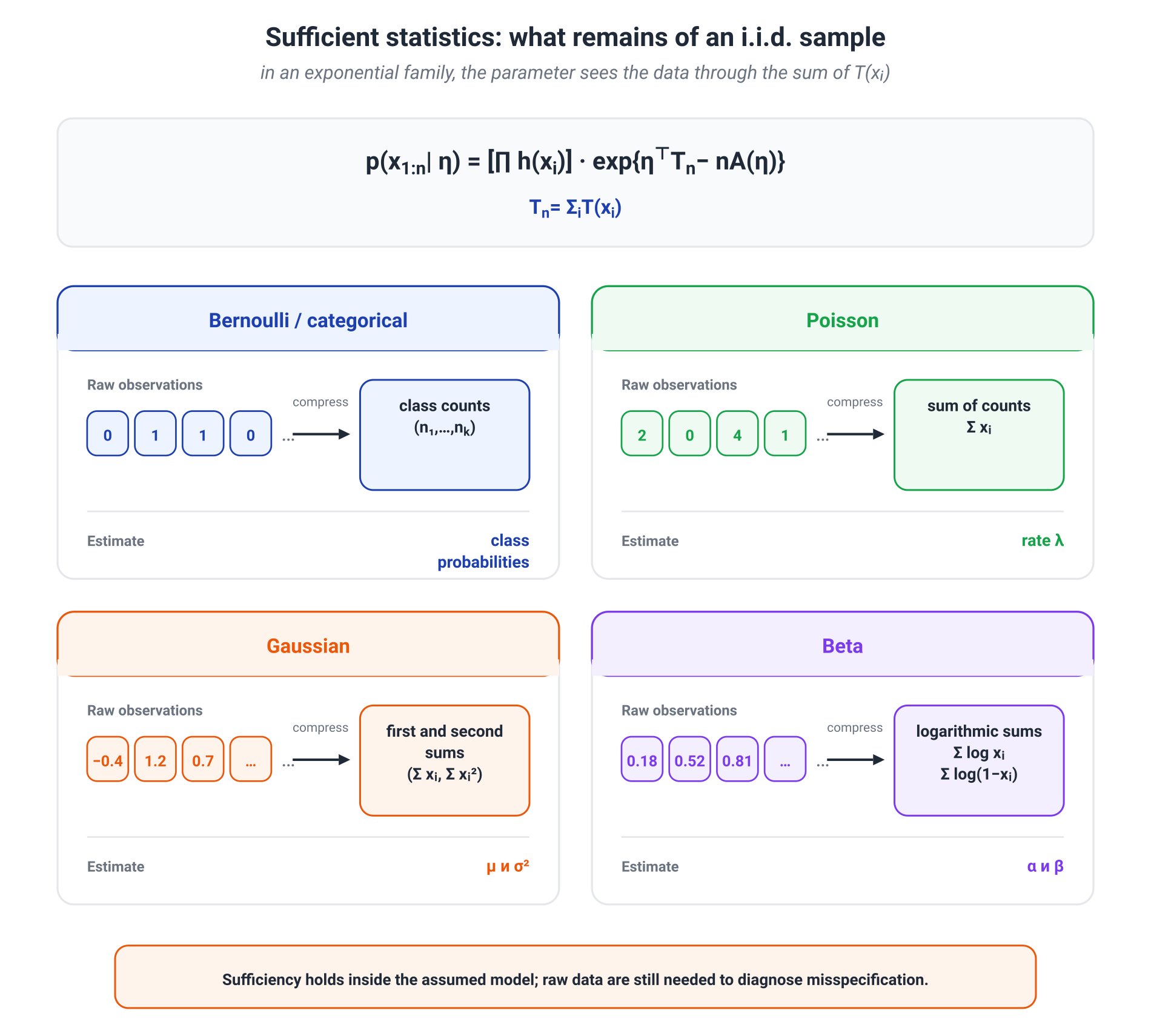
Sufficiency has a precise meaning: conditional on $T_n$, the distribution of the original sample does not depend on $\eta$. Once the statistic has been computed, the raw observations contain no further information about the parameter inside the assumed model.

The final phrase matters. Order, outliers, multimodality, or systematic dependence may be irrelevant for estimating a parameter inside the family yet remain exactly the evidence that the i.i.d. family is misspecified. A sufficient statistic compresses data relative to a specified inferential question; it is not a universally lossless representation of the dataset.

Maximum likelihood as matching mean statistics

Mean log likelihood is

$$\frac1n\log p(x_{1:n}\mid\eta) = \eta^\top\overline T -A(\eta) + \frac1n\sum_i\log h(x_i),$$

where

$$\overline T = \frac1n\sum_iT(x_i).$$

Up to a term independent of $\eta$, mean negative log likelihood is

$$\mathcal L_n(\eta) = A(\eta)-\eta^\top\overline T.$$

Its gradient is

$$\boxed{ \nabla\mathcal L_n(\eta) = \mathbb E_\eta[T(X)]-\overline T },$$

and its Hessian is

$$\nabla^2\mathcal L_n(\eta) = \operatorname{Cov}_\eta(T(X)) \succeq0.$$

If the family is minimal and a finite interior maximum-likelihood estimate exists, then

$$\boxed{ \mathbb E_{\widehat\eta}[T(X)] = \overline T }.$$

This is the exact scope of moment matching. Here “moments” means expectations of sufficient statistics:

• Bernoulli gives $\widehat p=\overline x$;
• Poisson gives $\widehat\lambda=\overline x$;
• categorical probabilities match class frequencies;
• the full Gaussian family matches empirical first and second moments;
• Beta and Gamma estimates match averages involving logarithms and are usually obtained numerically.

When no finite solution exists

Convex form does not guarantee that the optimum lies at a finite point of the natural parameter space.

• If every Bernoulli observation is one, the MLE has $\widehat p=1$, while $\widehat\eta\to+\infty$.
• If a class never appears in a categorical sample, its estimated probability lies on the boundary and the corresponding minimal log odds tend to $-\infty$.
• Under linear separability, unregularized conditional logistic regression may have no finite MLE.
• Regularization changes the stationarity condition, so exact empirical/model moment matching is offset by the penalty gradient.
• In a curved exponential family, where $\eta$ is constrained to a lower-dimensional nonlinear manifold, all coordinates of $T$ need not be matched independently.

These cases do not refute the geometry. They distinguish existence of a probability distribution, existence of a finite natural parameter, and existence of an interior MLE.

The Pitman–Koopman–Darmois theorem

So far we moved from exponential form to a sufficient statistic. Under standard regularity conditions, the Pitman–Koopman–Darmois theorem moves in the reverse direction:

For a regular dominated i.i.d. family with common parameter-independent support, the existence of a sufficient statistic whose dimension remains bounded as $n$ grows severely restricts the model and leads to finite-dimensional exponential form.

This is a structural theorem, not a model-selection recipe. Its assumptions do real work.

For example,

$$X_i\sim\operatorname{Uniform}(0,\theta)$$

has the one-dimensional sufficient statistic

$$\max_iX_i,$$

but its support $[0,\theta]$ depends on the parameter. The standard PKD theorem therefore does not apply.

Other nonregular cases—parameter-dependent support, degeneracy, some discrete settings, or failures of smoothness—also require a more careful formulation. The correct lesson is not that “any sufficient statistic proves exponentiality,” but that in a regular i.i.d. problem, compressing every sample size to a fixed number of coordinates is an exceptionally strong property.

Three connections, not one theorem

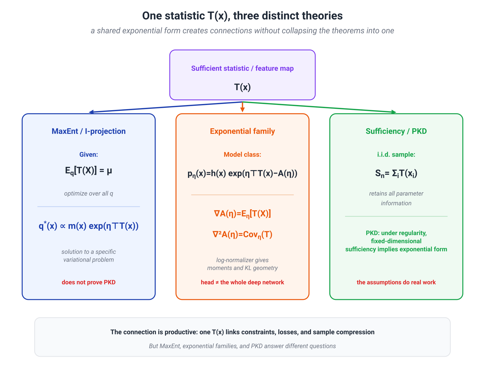
We can now assemble the picture without collapsing distinct statements.

1. MaxEnt / information projection. Optimizing over all distributions under constraints on means of $T(X)$ produces an exponential tilt of the base.
2. Exponential family. A parametric class is specified in advance as $h(x)e^{\eta^\top T(x)-A(\eta)}$; $A$ maps natural parameters to means and determines the class's KL geometry.
3. Sufficiency / PKD. For an i.i.d. sample, $\sum_iT(X_i)$ is sufficient, while under regularity the existence of a fixed-dimensional sufficient statistic is tightly connected to exponential form.

The same statistic $T(x)$ genuinely plays a central role in all three stories. That is why the connection is so productive in ML: it unifies probabilistic output heads, convex losses, statistic matching, and compact data summaries for parameter estimation.

The boundaries matter as well. MaxEnt does not prove PKD; PKD does not say that every convenient ML distribution was selected by maximum entropy; and an exponential-family output head does not make an entire deep network an exponential family in its weights.

The reusable skill after this section is simple:

Do not memorize the exponential family as a list of distributions. Learn to read a log density: support and base, sufficient statistics, natural parameters, log-partition function, and the domain on which it is finite.

8.12. Conclusion

We began in a setting where a few known averages were insufficient to recover a distribution. MaxEnt did not supply missing facts or guess a hidden truth. It did something more modest and more useful: among distributions genuinely compatible with the constraints, it selected the one closest to a reference.

The central construction of the module is

$$\boxed{ q^*(x) \propto m(x)e^{s(x)} }.$$

The meanings of the two components changed across sections:

This table explains the unity of the module better than any slogan. Constraints, scores, energies, and rewards enter log probability additively; exponentiation redistributes mass multiplicatively; the partition function reconciles local preferences into one distribution.

Shared algebra does not erase the differences among problems. In MaxEnt we optimize over distributions under specified moments. In an EBM, energy may be an arbitrary neural network with no explicit system of physical constraints. In DPO, the analytical Gibbs form enters the derivation of the loss, while a real policy remains restricted by parameterization and data. KL keeps a distribution near a reference but does not verify that the reward is true.

That is the balance needed in later modules: see the common construction clearly enough to transfer intuition, while retaining the conditions that keep the transfer from becoming a metaphor.

Module 9 changes the object of optimization. Instead of asking “which distribution should we choose?”, we ask “which representation should we preserve?” Information Bottleneck, rate–distortion, and variational autoencoders again turn learning into a trade-off—this time between retained information and the cost of representing it.

Primary sources

1. E. T. Jaynes, Information Theory and Statistical Mechanics, 1957, and Part II, Physical Review 108, 171.
2. A. Berger, S. Della Pietra, and V. Della Pietra, A Maximum Entropy Approach to Natural Language Processing, 1996.
3. J. Lafferty, A. McCallum, and F. Pereira, Conditional Random Fields: Probabilistic Models for Segmenting and Labeling Sequence Data, ICML 2001.
4. M. Wainwright and M. Jordan, Graphical Models, Exponential Families, and Variational Inference, 2008.
5. Y. LeCun et al., A Tutorial on Energy-Based Learning, 2006.
6. Y. Song et al., Score-Based Generative Modeling through Stochastic Differential Equations, 2021.
7. J. Schulman et al., Proximal Policy Optimization Algorithms, 2017.
8. R. Rafailov et al., Direct Preference Optimization: Your Language Model Is Secretly a Reward Model, 2023.
9. L. Gao, J. Schulman, and J. Hilton, Scaling Laws for Reward Model Overoptimization, 2022.
10. Y. Polyanskiy and Y. Wu, Information Theory: From Coding to Learning, 2025, sections on exponential families and information projection.
11. L. D. Brown, Fundamentals of Statistical Exponential Families, 1986.