Module 2. Entropy

How to read this module. The main route is §§2.1–2.4. Short proofs of the basic properties belong to the core: they expose the mechanism and will be used later. Two passages are marked as mathematical deep dives—the derivation of entropy rate and the derivative of entropy with respect to temperature. They can wait for a second pass. The engineering aside on speculative decoding is optional as well.

2.1. Entropy: the average bill for uncertainty

Consider two classifiers that choose the same class. The first returns

$q_A=(0.97,0.01,0.01,0.01),$

while the second returns

$q_B=(0.40,0.30,0.20,0.10).$

Their argmax decisions are indistinguishable: class 1 wins in both cases. The distributions themselves are not. The first concentrates almost all probability mass at one point; the second leaves several plausible alternatives alive. Entropy detects exactly this difference:

$H(q_A)\approx0.242\ \text{bits},\qquad H(q_B)\approx1.846\ \text{bits}.$

This is the first ML interpretation of entropy: it looks beyond the winner and measures the shape of the entire distribution.

Module 1 explained why the surprise of a single outcome should be logarithmic. We now take the next step. Let a discrete random variable $X$ have distribution $P$, with probabilities $p(x)$. Unless stated otherwise, alphabets in this module are finite, logarithms use base 2, and information is measured in bits.

The surprisal, or self-information, of a particular outcome $x$ is

$i_P(x)=-\log_2 p(x).$

Shannon entropy is expected surprisal:

$$H_P(X) =\mathbb E_{X\sim P}[i_P(X)] =-\sum_{x\in\mathcal X}p(x)\log_2 p(x).$$

The convention $0\log0:=0$ is defined by continuity, because $u\log u\to0$ as $u\to0^+$.

There is a simple way to read the formula. Imagine that the source sends a bill for every realized outcome: $-\log_2 p(x)$ bits. A rare outcome is expensive but occurs rarely; a common outcome is cheap but arrives often. Entropy is the average bill before the result is known.

One more scale is often useful. The quantity

$N_{\mathrm{eff}}=2^{H(P)}$

indicates how many equally likely outcomes would correspond to the same entropy. For a general distribution this is an effective number: it need not be an integer and is not the literal support size. An entropy of 3 bits, for example, carries the same uncertainty as eight equiprobable choices.

Property 1. From certainty to the uniform distribution

For a distribution on $n$ possible outcomes,

$0\le H(X)\le\log_2 n.$

The lower bound is attained when the outcome is effectively predetermined. The upper bound is attained when all $n$ outcomes are equally likely. Entropy therefore places certainty and complete symmetry between alternatives at opposite ends of the scale.

Nonnegativity. For every outcome with $p(x)>0$,

$-\log_2 p(x)\ge0.$

Every nonzero term in the expectation is therefore nonnegative. Equality $H(X)=0$ is possible only when one outcome has probability 1. $\blacksquare$

Maximum. Zero probabilities require a little care. Let the positive support be

$\mathcal S=\{x:p(x)>0\},\qquad m=|\mathcal S|\le n.$

For the concave logarithm, Jensen’s inequality reads

$$\sum_x w_x\log_2 a_x\le\log_2\!\left(\sum_x w_xa_x\right).$$

Therefore

$$\begin{aligned} H(X) &=\sum_{x\in\mathcal S}p(x)\log_2\frac1{p(x)}\\ &\le\log_2\!\left(\sum_{x\in\mathcal S}p(x)\frac1{p(x)}\right) =\log_2 m \le\log_2 n. \end{aligned}$$

The first inequality becomes an equality only when $p(x)$ is constant on the support. Reaching $\log_2 n$ further requires all $n$ outcomes to lie in that support. The unique maximizer is therefore the uniform distribution on the full alphabet. $\blacksquare$

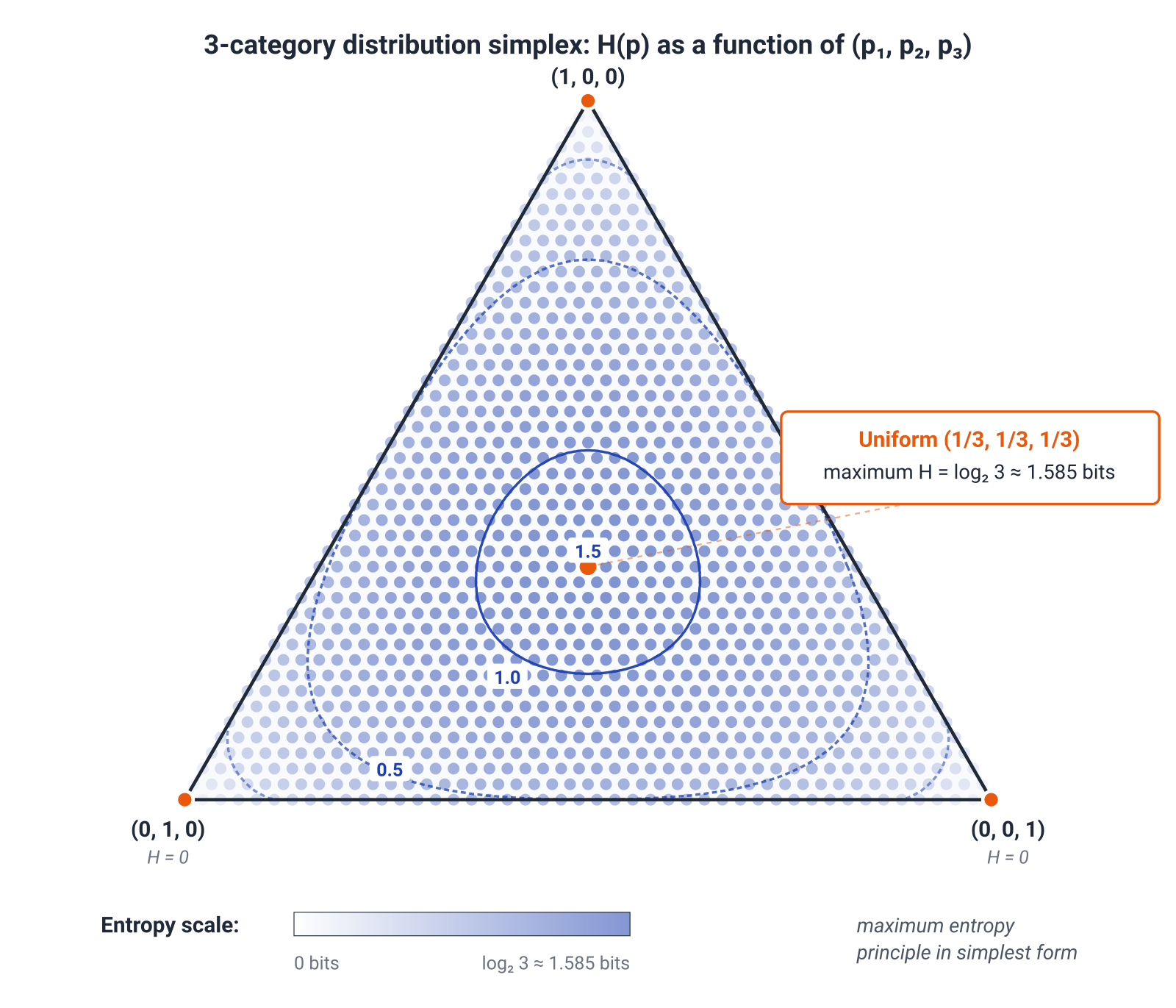
This is the maximum-entropy principle in its simplest form: when only the set of possible outcomes is known, the uniform distribution introduces no unsupported preference among them. In Module 8 we will add moment constraints and see how the same principle produces nonuniform exponential distributions and softmax.

The bounds are also a useful engineering test. If code for a distribution over a vocabulary of size $n$ returns negative entropy or a value above $\log_2 n$, the problem is not a subtle interpretation. The computation is wrong.

Property 2. Concavity: forgetting the mixture component adds uncertainty

Suppose we have two distributions $p$ and $q$. Before generating an observation, we choose the first with probability $\lambda$ and the second with probability $1-\lambda$. If we then forget which component was selected, the observed law is the mixture

$r=\lambda p+(1-\lambda)q.$

Entropy satisfies

$H(r)\ge\lambda H(p)+(1-\lambda)H(q).$

Losing the information about which component generated the example cannot reduce average uncertainty. This result will keep returning—in mixtures, latent-variable models, ensembles, and mutual information.

Proof. The function

$\varphi(u)=-u\log_2u$

has, for $u>0$,

$\varphi''(u)=-\frac1{u\ln2}<0.$

After the continuous extension $\varphi(0)=0$, it is strictly concave on $[0,1]$. Since

$H(p)=\sum_i\varphi(p_i),$

entropy is concave on the probability simplex. For $0<\lambda<1$, equality holds only when $p=q$. $\blacksquare$

It is easy to claim slightly more than the inequality gives. The entropy of a mixture is no smaller than the average entropy of its components, but it need not exceed every component. Mixing a uniform distribution with a point mass still produces a distribution less entropic than the uniform component.

2.2. The chain rule: splitting one bill across tokens

A sequence can receive one bill for the whole outcome, or the bill can be paid in stages. The chain rule says that, with the correct conditioning, the total is unchanged.

Let $X$ and $Y$ have joint distribution $p(x,y)$. Their joint entropy is

$H(X,Y)=-\sum_{x,y}p(x,y)\log_2p(x,y).$

The conditional entropy of $Y$ after observing $X$ is

$$\begin{aligned} H(Y\mid X) &=\sum_{x:p(x)>0}p(x)H(Y\mid X=x)\\ &=-\sum_{x,y}p(x,y)\log_2p(y\mid x). \end{aligned}$$

The key word is average. $H(Y\mid X)$ averages residual uncertainty over possible values of $X$. It is not the same object as $H(Y\mid X=x_0)$ for one particular event. For values with $p(x)=0$, the conditional distribution may be assigned arbitrarily because it receives zero weight.

The chain rule

$H(X,Y)=H(X)+H(Y\mid X).$

Read the equation before proving it. We first pay $H(X)$ bits on average to learn $X$. Once $X$ is known, an average of $H(Y\mid X)$ bits remains for $Y$. Together these are exactly the same bill as describing the pair $(X,Y)$ directly.

Proof. On the positive support,

$p(x,y)=p(x)p(y\mid x).$

The logarithm turns the product into a sum:

$$\begin{aligned} H(X,Y) &=-\sum_{x,y}p(x,y)\log_2\bigl(p(x)p(y\mid x)\bigr)\\ &=-\sum_{x,y}p(x,y)\log_2p(x) -\sum_{x,y}p(x,y)\log_2p(y\mid x)\\ &=H(X)+H(Y\mid X). \end{aligned} \qquad\blacksquare$$

The order may be reversed:

$H(X,Y)=H(Y)+H(X\mid Y).$

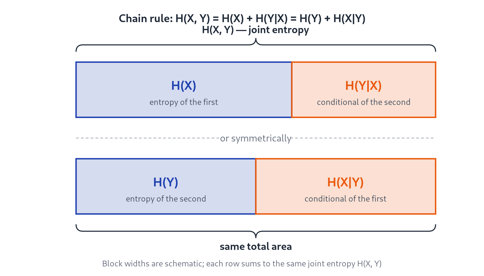
Applying the rule inductively to a sequence gives

$$H(X_1,\ldots,X_n) =\sum_{i=1}^nH(X_i\mid X_1,\ldots,X_{i-1}) =\sum_{i=1}^nH(X_i\mid X_{<i}).$$

Here is the memorable version: the chain rule is the bookkeeping of autoregression. Joint uncertainty in a sequence decomposes into the residual uncertainty of each next element after the prefix is known. If q is almost always followed by u, the context makes the second character cheap. If the continuation is genuinely open-ended, the bill remains large.

Source and model: one factorization, two different bills

The phrase “the chain rule literally describes what a language model does” is almost right, but it needs one crucial fork.

Suppose data are generated by a distribution $P$:

$p(x_{1:n})=\prod_{i=1}^np(x_i\mid x_{<i}).$

Then the chain rule decomposes the entropy of the source itself:

$H_P(X_{1:n})=\sum_{i=1}^nH_P(X_i\mid X_{<i}).$

An autoregressive model defines its own distribution $Q_\theta$:

$q_\theta(x_{1:n})=\prod_{i=1}^nq_\theta(x_i\mid x_{<i}).$

For one observed sequence, the model bill also decomposes token by token:

$$-\log_2 q_\theta(x_{1:n}) =\sum_{i=1}^n-\log_2 q_\theta(x_i\mid x_{<i}).$$

After averaging over data from $P$, however, we do not automatically obtain $H(P)$. We obtain the cross-entropy of the source relative to the model:

$H(P,Q_\theta)=\mathbb E_{X\sim P}\bigl[-\log_2q_\theta(X)\bigr].$

The two quantities agree only when the model conditionals equal the source conditionals $P$-almost surely. Module 3 will expose the difference in one line:

$H(P,Q)=H(P)+D_{\mathrm{KL}}(P\|Q).$

For now, keep the interpretation. The chain rule really does explain why a language-model loss adds across tokens. It does not say that every such loss is already the intrinsic entropy of the source.

Conditioning reduces entropy—but only on average

Context helps on average:

$H(Y\mid X)\le H(Y),$

with equality if and only if $X$ and $Y$ are independent.

Proof. The marginal distribution of $Y$ is a mixture of conditional distributions:

$p_Y=\sum_xp(x)p_{Y\mid X=x}.$

By concavity of entropy,

$$H(Y) =H\!\left(\sum_xp(x)p_{Y\mid X=x}\right) \ge\sum_xp(x)H(Y\mid X=x) =H(Y\mid X).$$

Strict concavity implies that equality holds only when all positive-weight conditionals are identical to $p_Y$, which is exactly independence. $\blacksquare$

Subadditivity follows immediately:

$H(X,Y)\le H(X)+H(Y),$

with equality exactly under independence.

The boundary of the claim is compact but important. For one particular value $x_0$, it may happen that

$H(Y\mid X=x_0)>H(Y).$

A specific observation can reveal a more ambiguous regime even though observing $X$ reduces uncertainty on average. Exercise 3 builds such an example without tricks.

2.3. From a coin to language: entropy rate

A coin as a laboratory

For a coin with head probability $p$, entropy is

$h_2(p)=-p\log_2p-(1-p)\log_2(1-p).$

Lowercase $h_2$ is customary for the binary entropy function and also helps distinguish it from Rényi entropy of order 2, often denoted $H_2$.

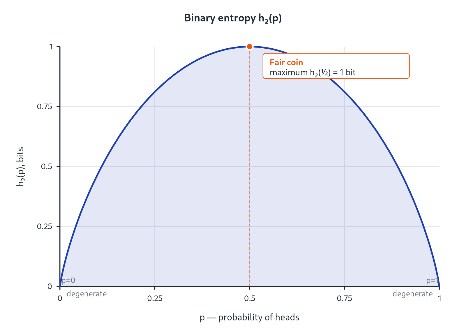
The graph tells the whole story. At $p=0$ or $p=1$, the next toss is already known and entropy is zero. At $p=1/2$, neither outcome is preferred, so uncertainty is maximal at one bit. Exercise 1 asks you to verify the derivatives and strict concavity.

Text, however, is not a bag of independently drawn characters. If we count character frequencies and then shuffle a string, we preserve its one-character entropy while destroying words, syntax, and topic. Language therefore needs a quantity that accounts for dependence on context.

The main result for a source with memory

Let $(X_t)_{t\ge1}$ be a stationary process over a finite alphabet: the distribution of every finite block is invariant under a shift in time. Write the residual uncertainty of the next symbol given a context of length $n-1$ as

$h_n=H(X_n\mid X_1,\ldots,X_{n-1}),\qquad h_1=H(X_1).$

Longer context does not increase this quantity on average, and the limit

$$\boxed{ h =\lim_{n\to\infty}H(X_n\mid X_1,\ldots,X_{n-1}) =\lim_{n\to\infty}\frac1nH(X_1,\ldots,X_n) }$$

exists. It is the entropy rate of the source.

This is the precise version of “how many genuinely new bits the next symbol contributes, on average, when the entire past is available.” One-symbol entropy asks about a character without context. Entropy rate asks about the irreducible remainder after the source's dependencies have been used.

Mathematical deep dive: why the limit exists. On a first reading, you may continue directly to Shannon's experiment below.

By “conditioning reduces entropy” and stationarity,

$$\begin{aligned} h_{n+1} &=H(X_{n+1}\mid X_1,\ldots,X_n)\\ &\le H(X_{n+1}\mid X_2,\ldots,X_n)\\ &=H(X_n\mid X_1,\ldots,X_{n-1})=h_n. \end{aligned}$$

Thus $(h_n)$ is non-increasing and bounded below by zero, so it converges. The chain rule gives

$$\frac1nH(X_1,\ldots,X_n)=\frac1n\sum_{i=1}^nh_i.$$

The Cesàro means of a convergent sequence have the same limit as the sequence itself, yielding both expressions in the box.

The phrase “bits per character” now has a rigorous object behind it, but it also has conditions: the source, alphabet, stationarity assumption, and preprocessing rules must be specified. Without them, “the entropy of English” sounds meaningful but does not denote a single universal constant.

Shannon asks a person to act as a language model

In his 1951 paper Prediction and Entropy of Printed English, Shannon used a 27-symbol alphabet: 26 letters plus space. Successive approximations showed how context removes uncertainty:

The most beautiful part begins where short $n$-gram tables stop being enough. A subject saw the preceding text and tried to guess the next character. If the first guess failed, they tried a second, then a third, until the correct character was found. The rank of the successful guess turned human knowledge of words, grammar, clichés, and topic into quantitative constraints on conditional entropy.

With contexts on the order of one hundred preceding characters, Shannon's final table produced roughly 1.3 bits/symbol as an upper bound and 0.6 bits/symbol as a lower bound. His conclusion was deliberately cautious: for ordinary literary English, long-range effects reduce entropy to a magnitude on the order of one bit per letter.

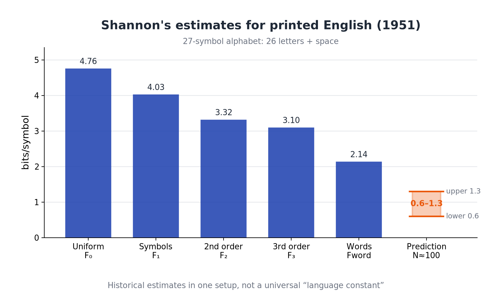
Why is the experiment still striking? Uniform choice among 27 symbols costs 4.76 bits. A human predictor, using structure tens of positions back, discovers that most of that bill is predictable. Syntax, fixed expressions, and topic cease to be an abstract “meaning” and become statistical constraints on the continuation.

The strength of the result does not require turning 1 bit into a physical constant. Shannon's sample was small; rare guess ranks were hard to estimate; a person is not an optimal predictor; newswire, scientific prose, and poetry are different sources. The interval $0.6$–$1.3$ is a historical estimate under a particular experiment, not a lower limit for every file written in English.

Under the standard assumptions of the source coding theorem, entropy rate sets the asymptotic limit for lossless compression. That theorem is the subject of Module 6. For now, note what the theorem is about: a specified stochastic source, not the word “language” without a data model.

A modern language model as a compressor

An autoregressive LLM performs a task closely related to Shannon's experiment: given a prefix, it assigns probabilities to possible continuations. Feed those probabilities to arithmetic or range coding and model NLL becomes, up to a small coding overhead, an achievable compressed length.

This gives a precise and useful picture:

• a better model on a held-out corpus will usually pay fewer bits and serve as a better compressor;
• its cross-entropy remains an upper bound on source entropy under the same setup;
• approaching Shannon's historical estimate is interesting, but matching numbers obtained from different corpora, alphabets, and protocols proves nothing by itself.

If $Q$ assigns positive probability to every sequence that can occur under $P$, then for every $n$,

$$H_P(X_{1:n}) \le \mathbb E_P[-\log_2q(X_{1:n})].$$

After division by $n$, the model coding rate may approach entropy rate from above. The gap is the price of model mismatch; in the next module it will acquire the name KL divergence.

The inequality concerns an expectation over the source. For example, with $P=Q=\operatorname{Bernoulli}(0.9)$, entropy is about $0.469$ bits, while a corpus consisting of one outcome $1$ has NLL only $-\log_2 0.9\approx0.152$ bits. That corpus occurs with probability $0.9$: one measurement can lie below entropy without violating the theorem.

2.4. How to read entropy in a language model

In ML, the word “entropy” is used for several related numbers that answer different questions. Before interpreting one, ask two things: whose distribution appears inside the logarithm, and under which distribution is the average taken?

Many overstrong conclusions come from silently moving between these rows.

Predictive entropy: how broad is the model's menu?

For a fixed context $c=x_{<t}$, the model returns a distribution $q_\theta(v\mid c)$ over vocabulary $\mathcal V$. Its entropy is

$$H_\theta(c) =-\sum_{v\in\mathcal V}q_\theta(v\mid c)\log_2q_\theta(v\mid c).$$

A low value means that probability mass is concentrated on a small number of tokens. A high value means that many continuations share non-negligible mass. The quantity

$2^{H_\theta(c)}$

is a useful “effective menu size”: it is literally the number of alternatives for a uniform distribution and an entropy-equivalent number for a general one.

This is a useful local diagnostic. It can reveal an abrupt branching point, excessive concentration, a behavior change after fine-tuning, or an unusual part of a sequence. But entropy answers a question about concentration, not factual truth. A model can be confidently wrong; high entropy may reflect genuine multiplicity rather than confusion. Calibration and the separation of epistemic from aleatoric uncertainty require additional structure and data.

In particular, do not confuse predictive entropy with test NLL. A model can sharpen its distribution, reduce $H(Q_\theta(\cdot\mid c))$, and simultaneously increase loss on the observed token if mass moved in the wrong direction.

Temperature: one case where the direction is exact

Let $z_v$ be fixed logits and

$$q_T(v)=\frac{\exp(z_v/T)}{\sum_u\exp(z_u/T)},\qquad T>0.$$

Here we can make a statement without empirical qualifiers: for fixed logits, increasing temperature cannot decrease entropy. Low temperature magnifies logit differences and concentrates mass near maxima; high temperature smooths them.

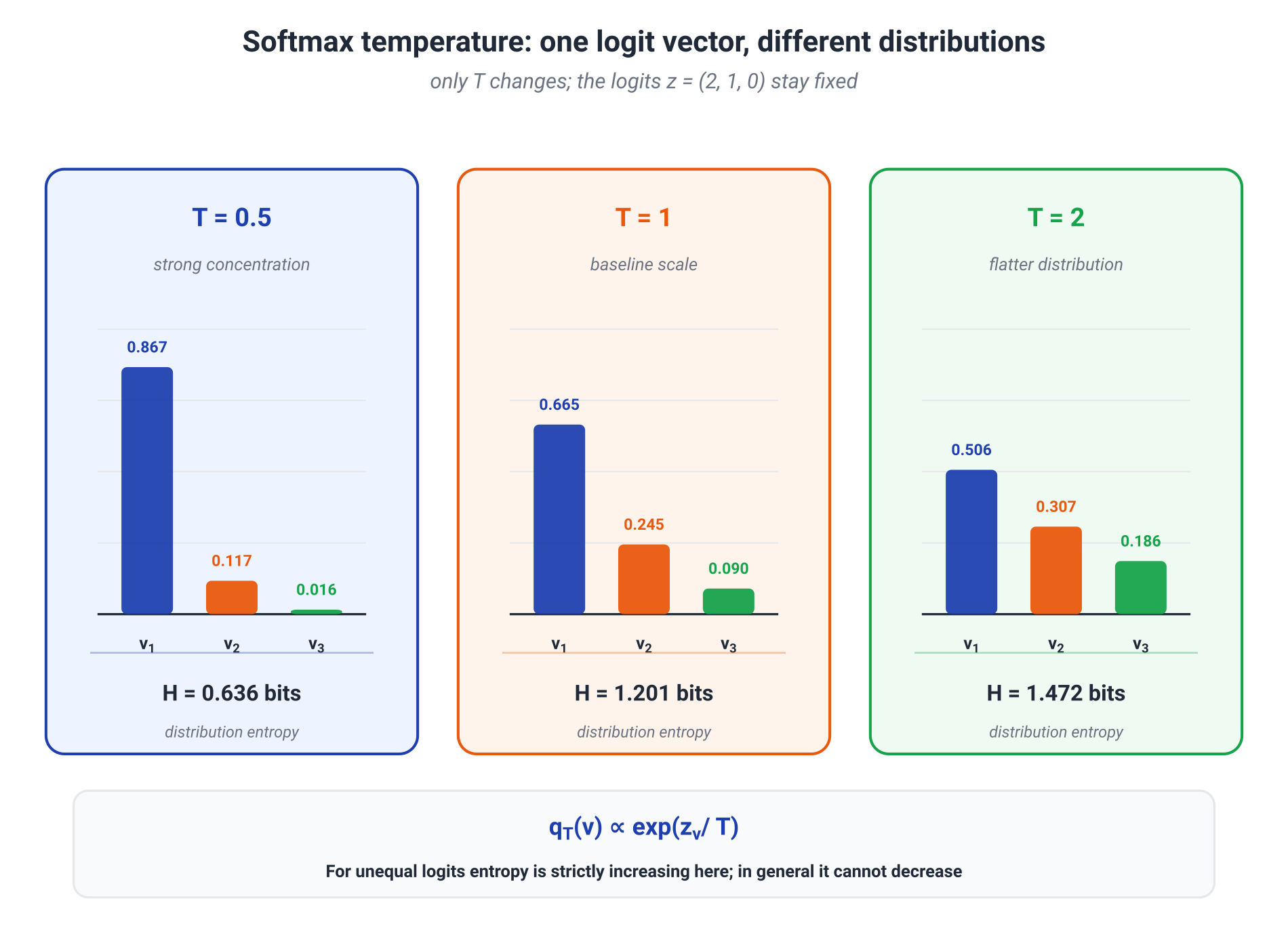
If one token uniquely maximizes the logit, entropy tends to zero as $T\to0$. If $r$ tokens share the maximum, the limit is $\log_2r$. As $T\to\infty$, the distribution tends to uniform over the vocabulary and

$H(q_T)\to\log_2|\mathcal V|.$

Thus, when the logits are not all equal, every target entropy strictly between the two limiting values determines a unique temperature.

Mathematical deep dive: the derivative with respect to temperature. Let $\beta=1/T$ and temporarily measure entropy in nats. For $Z(\beta)=\sum_v e^{\beta z_v}$,

$H(q_T)=\log Z(\beta)-\beta\,\mathbb E_{q_T}[z].$

Since

$\frac{d}{d\beta}\mathbb E_{q_T}[z]=\operatorname{Var}_{q_T}(z),$

we obtain

$$\frac{dH}{d\beta}=-\beta\operatorname{Var}_{q_T}(z), \qquad \frac{d\beta}{dT}=-\frac1{T^2},$$

and therefore

$$\frac{d}{dT}H(q_T) =\frac{\operatorname{Var}_{q_T}(z)}{T^3}\ge0.$$

For entropy in bits, divide the right-hand side by $\ln2$.

The monotonicity statement applies specifically to pure temperature scaling with fixed logits. Top-$k$, top-$p$, min-$p$, and other filters first alter support or relative weights and then renormalize. They are different transformations and cannot inherit the temperature result without a separate argument.

Post-training: a useful hypothesis, not a universal law

The popular claim “instruction tuning lowers entropy” has a plausible empirical core: SFT, RLHF, or DPO teach a model to prefer particular response formats. On a specific set of instruction-following prompts, this may concentrate probability mass, lower mean predictive entropy, and reduce diversity. The model becomes less likely to continue the prompt as an arbitrary web fragment and more likely to adopt the expected assistant role.

That conclusion does not follow from the label instruct itself. Post-training changes logits in a context-dependent way. It can increase entropy where the base model was overconfident in an undesirable continuation and decrease it where preferences impose a narrow format. Mode collapse is a possible failure mode under aggressive optimization, not the definition of RLHF.

The right engineering question is therefore not “do instruct models have lower entropy?” but:

On a fixed prompt set, with the same tokenizer and before sampling filters, how did the token distributions change after post-training?

That is a measurable experiment rather than a dispute between slogans.

Engineering aside: why entropy alone is insufficient for speculative decoding

Consider two distributions over tokens a and b:

$p=(0.9,0.1),\qquad q_1=(0.9,0.1),\qquad q_2=(0.1,0.9).$

The distributions $q_1$ and $q_2$ have the same entropy. Yet the first matches $p$, while the second nearly swaps its mass. For exact speculative decoding, that difference is decisive.

In the basic one-step construction of exact speculative decoding, the mean acceptance probability for a draft token is

$$\alpha =\sum_v\min\{p(v),q(v)\} =1-\operatorname{TV}(p,q),$$

where

$\operatorname{TV}(p,q)=\frac12\sum_v|p(v)-q(v)|.$

For $q_1$, $\alpha=1$; for $q_2$, it is only $0.2$, despite equal entropies. The lesson extends beyond this algorithm: entropy compresses a distribution into one number and discards information about where its mass lies. When an engineering problem depends on agreement between two distributions, a measure of their distance or overlap is needed—not the entropy of either distribution in isolation.

Cross-entropy and perplexity: the model's bill on data

For a tokenized test sequence $x_{1:n}$, define mean loss using logarithm base $b$:

$$\widehat L_b =-\frac1n\sum_{i=1}^n\log_bq_\theta(x_i\mid x_{<i}).$$

This is empirical cross-entropy, or average NLL per token under the chosen normalization. Perplexity is

$\operatorname{PPL}=b^{\widehat L_b}.$

If loss is measured in nats, $\operatorname{PPL}=e^{\widehat L}$; if in bits, $\operatorname{PPL}=2^{\widehat L_2}$. Interpreting perplexity as an “effective number of equally likely alternatives” is exact for a uniform distribution and a useful equivalent scale more generally. It does not mean that the model literally chose from an integer number of candidates at every step.

Perplexity depends on tokenization: different tokenizers divide the same text into different events. It is therefore safest to compare PPL on the same corpus, with the same tokenizer and evaluation protocol. Bits per character or per byte use an external normalization unit and make comparisons easier, but they do not remove dependence on the model, context, preprocessing, and data composition.

The same distinction matters for scaling laws. They describe empirical decreases in test cross-entropy over the ranges of scale that were studied. This is a strong statement about models and data, but not a proof that an extrapolated asymptote must equal a universal entropy of language.

At this point, it is useful to compress the module to one question. When you encounter “entropy” in an ML paper or dashboard, ask: is the model distribution evaluating itself, is the model being evaluated on data, or are we talking about the unknown source? The formulas are related; the scientific conclusions are not interchangeable.

2.6. References and primary sources

1. C. E. Shannon, A Mathematical Theory of Communication, 1948—the original formulation of entropy, coding, and noisy channels.
2. C. E. Shannon, Prediction and Entropy of Printed English, 1951—the primary source for the English-guessing experiments.
3. T. M. Cover and J. A. Thomas, Elements of Information Theory, 2nd ed., 2006—entropy properties, the chain rule, and entropy rate.
4. D. J. C. MacKay, Information Theory, Inference, and Learning Algorithms, 2003—an intuitive, ML-oriented treatment.
5. Y. Polyanskiy and Y. Wu, Information Theory: From Coding to Learning, 2025—a modern rigorous treatment.
6. A. Holtzman et al., The Curious Case of Neural Text Degeneration, 2019—temperature, truncation-based decoding, and the shape of language-model distributions.
7. Y. Leviathan, M. Kalman, and Y. Matias, Fast Inference from Transformers via Speculative Decoding, ICML 2023—exact speculative decoding and draft-token acceptance.
8. G. Delétang et al., Language Modeling Is Compression, ICLR 2024—language-model cross-entropy as a coding bill.
9. J. Kaplan et al., Scaling Laws for Neural Language Models, 2020—empirical scaling laws for test cross-entropy.