Module 13. Reasoning in LLMs: computation, search, and information
How to read this module. This is the capstone of the course. The main route is §§13.1–13.10: what changes when a model receives more compute at inference time; why intermediate steps can help without introducing new data; how to allocate a budget between one long trajectory, multiple candidates, and verification; when context and tools genuinely add information; and how to evaluate the resulting system without conflating quality with cost. §13.11 is a mathematical deepening on stepwise information gain and sequential expressivity. It can be left for a second pass.
13.1. What changes when a model “thinks longer”
Consider the same model and the same prompt. In the first regime, the model immediately emits a short answer. In the second, it writes several dozen intermediate steps before answering. In the third, it constructs multiple solutions, runs code, observes test results, and selects a candidate.
The weights have not changed. Neither has the original prompt. Yet performance may differ substantially. What did the extra computation actually buy?
The word reasoning is often used for several different phenomena at once: a multistep task, a visible chain of thought, a search procedure, tool use, or simply a correct answer. That is too imprecise for engineering analysis. We will separate five objects.
- Sequential computation. The task requires a series of dependent operations: arithmetic, proof construction, debugging, or planning.
- Intermediate state. The model stores partial results in a visible chain of thought (CoT), a hidden scratchpad, or some other internal state.
- Search. The system considers several candidates, branches, backtracks, or reallocates its compute budget.
- External observation. The system receives a search result, code output, test result, measurement, or environmental response.
- Outcome quality. A predefined metric improves: accuracy,
pass@k, log loss, robustness, or solution cost.
These objects are related but not identical. A long chain can be wrong. A correct answer does not prove that the visible prose was the causal mechanism. Search may improve an answer without producing one elegant trajectory. A calculator can sharply improve accuracy while adding no new fact about the world. A retrieval system, by contrast, may supply information that was absent from the prompt.
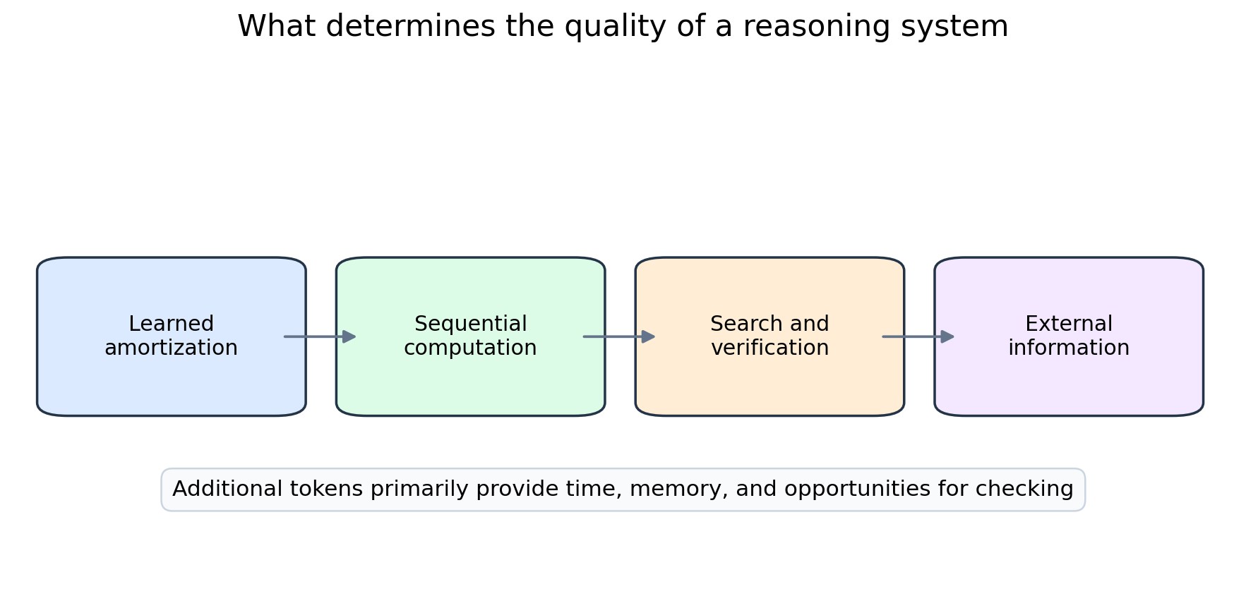
Chain-of-thought prompting showed that step-by-step demonstrations can substantially improve large language models on arithmetic, symbolic, and some commonsense tasks. Later, compute per query became an explicit optimization resource: a system can generate more tokens, sample several trajectories, consult a verifier, or interact with an environment.
The central question of this module is therefore:
What does additional computation purchase: new evidence, richer computation over existing evidence, or broader search over possible solutions?
The answer depends on the system architecture. We begin with three basic regimes.
13.2. Amortization, scratchpads, and search
Pretraining can be viewed as amortizing computation. A huge training cost compiles statistical regularities, facts, heuristics, and fragments of algorithms into parameters. At inference time, the model applies this accumulated structure to a new prompt.
An amortized answer
In the simplest regime, the model receives a prompt and emits an answer directly:
Most of the work was already paid for during training. This is fast, but the per-instance computational budget is small. If the required procedure was not compiled into a reliable heuristic, the model may settle on a locally plausible continuation too early.
A sequential scratchpad
Now let the model generate intermediate tokens
before producing the answer :
Each token supplies another sequential application of the model and another place to record an intermediate result. A scratchpad can therefore increase the system’s effective computational depth without changing its parameters.
The qualifier can matters. A token is not automatically a useful operation. The model may record a correct partial result, repeat itself, or send the computation down a bad branch. Extra budget creates an opportunity for work; it does not guarantee that the work is valuable.
Explicit search and interaction
In the third regime, the system considers alternatives and receives feedback. Examples include:
- self-consistency: sample several trajectories and vote over answers;
- best-of-: generate several candidates and rank them with a verifier;
- beam or tree search;
- Tree of Thoughts: branch, evaluate partial states, and backtrack;
- calls to an interpreter, calculator, or test suite;
- an agent loop of action, observation, and revised action.
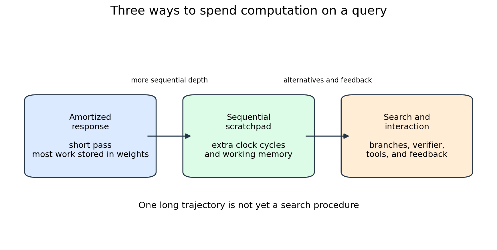
One long chain is not yet a search procedure. Search begins when the system preserves alternatives, compares them, can abandon an early choice, or receives a signal from the environment.
A useful boundary between amortization and search
At one end lies a model that immediately returns a learned response. At the other lies a system that explores a fresh solution space for every prompt. Between them are many intermediate regimes: a short scratchpad, a handful of samples, local verification, or an adaptive budget.
This spectrum is more useful than a literal analogy to Solomonoff induction. The universal predictor from Module 10 mixes over all computable explanations and enjoys special theoretical guarantees. An ordinary LLM does not implement that mixture and does not inherit those guarantees. The distinction between an amortized heuristic and computation devoted to the current instance, however, is real and useful.
13.3. Why intermediate tokens can help
The most direct explanation is computational. Autoregressive generation lets a model apply the same network block repeatedly while carrying forward an expanding state.
Consider parity of bits:
A linear classifier on the original bit vector cannot solve parity. A single bit of working memory is enough, however:
After steps,
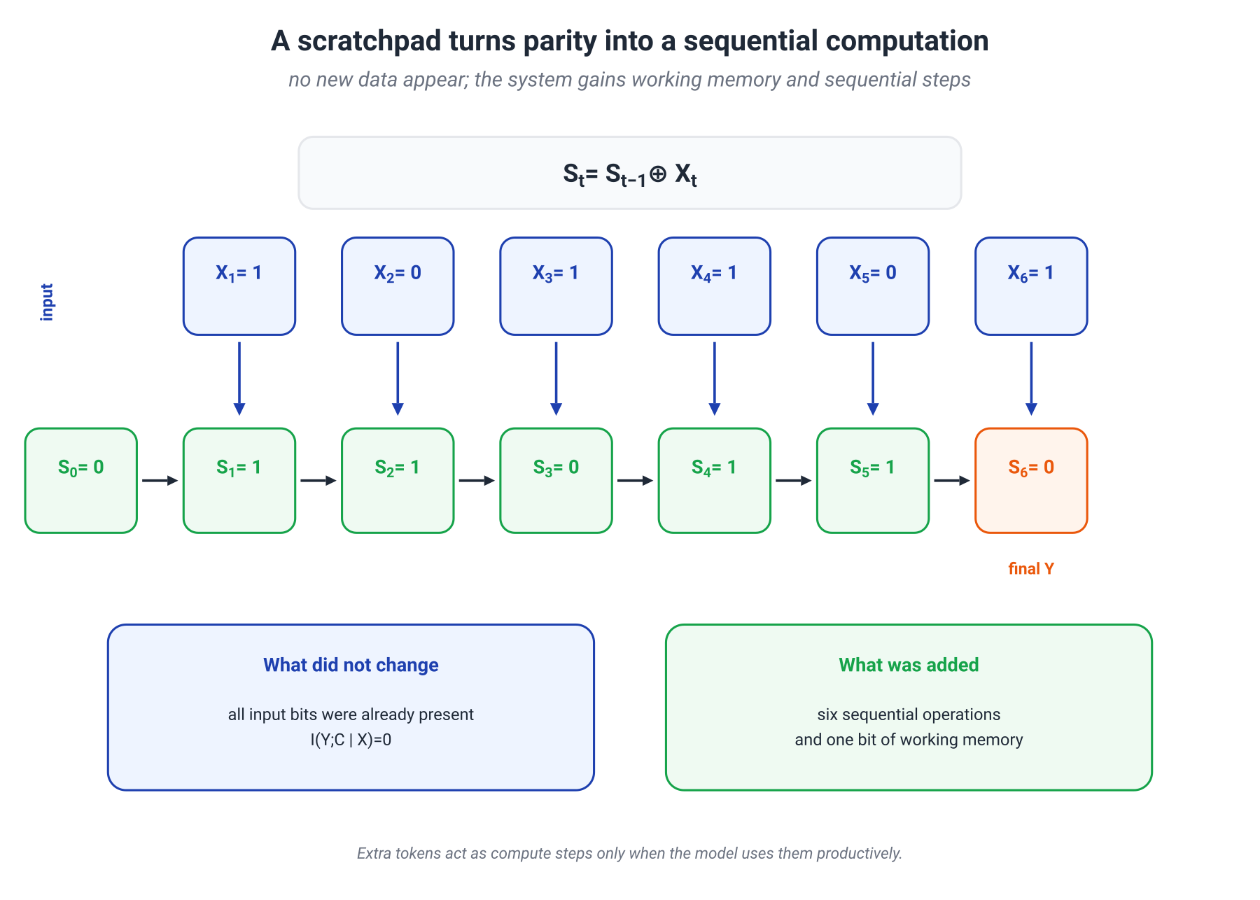
No new data were added to . The procedure changed: a restricted one-shot readout was replaced by a sequential algorithm.
Here the extra tokens act as computational clock cycles and working memory, not as new observations.
This is more than an analogy. Under carefully specified computational assumptions, formal results show that intermediate CoT steps enlarge the class of serial computations available to a decoder-only Transformer. For example, with particular restrictions on depth, precision, and representation size, CoT steps can implement sequential circuits of size on the order of . This is not a universal theorem about every modern LLM, but it supports the mechanism: sequential decoding can add computational expressivity.
When a long scratchpad is most likely to help
The gain is most natural when a task:
- decomposes into dependent subtasks;
- requires intermediate values to be retained;
- admits local checks;
- is sensitive to an early branch choice;
- contains a procedure that is hard to compress into one local transition.
For a simple factual query, a long chain may only increase cost and create more places to make mistakes. Quality therefore need not be monotone in token count. The relevant resource is not text volume by itself, but useful computation performed within that volume.
13.4. New information or new computation?
We can now state the central exact result of the module.
Let , where is the complete task available to the model and is the correct answer. A fixed model constructs an internal chain from and private randomness :
Then
is a Markov chain. Hence
and
Short proof
By construction, once the input is known, the distribution of the chain does not depend on the correct answer:
Thus and are conditionally independent given , so . The remaining identities follow from the definition of conditional mutual information and the chain rule.
Read in words:
An internally generated chain tells an ideal observer no new fact about the correct answer beyond the complete input. It reorganizes information that was already available.
Why can a real model still become more accurate? Because a real model is not an ideal Bayesian observer that instantly computes . Its output is constrained by architecture, depth, and learned procedure. A scratchpad changes the available computational path and can make the target function easier for a downstream readout to access.
Define the model log loss after steps as
This loss may decrease because the model uses its intermediate results more effectively. That is a reduction in model loss, not in the source quantity . Even monotonicity is not guaranteed for a particular model: a bad intermediate step can raise the loss.
When new information really appears
Suppose that after an internal step the system receives an observation : a retrieval result, database response, sensor reading, hidden test, or environmental reaction. Then
The final term may be positive. The system is no longer merely computing; it is obtaining evidence.
A useful boundary case is a calculator. If all operands are already present in the prompt and the answer is deterministic, the calculator need not add Shannon information about the answer. It supplies a reliable computational primitive. Retrieval from an external database or a measurement of the environment, by contrast, may genuinely introduce evidence absent from the prompt.
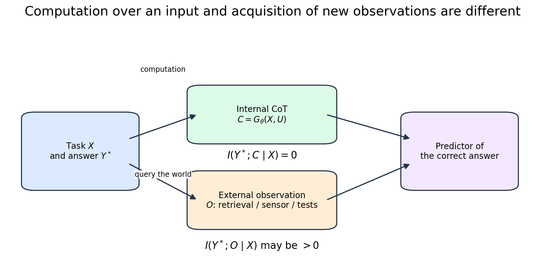
The resulting map is simple:
| System component | What it primarily contributes |
|---|---|
| model parameters | amortized knowledge and procedures |
| intermediate tokens | sequential depth and working memory |
| multiple candidates | search breadth |
| verifier | selection among discovered candidates |
| computational tool | a more reliable operation on existing data |
| retrieval, sensor, or environment | potentially new information |
13.5. What can be measured along a trajectory?
The phrase “this step added information” may refer to several different quantities. If they are not separated, the same curve is asked to represent computational progress, model confidence, and the true uncertainty of the task.
True information gain
If is a random intermediate state, then
measures the additional information about the correct answer in the new state after the old state is known. The quantity is meaningful only after the states and the distribution over tasks and trajectories have been defined.
For the complete internal context
with no external observations,
So a literal claim that every internal token contributes new bits about the answer is false in this model.
Improvement in an auxiliary predictor
A practical alternative is to train a separate predictor to recover the answer from the state after step , and measure held-out cross-entropy:
If it decreases, the state has become more useful to the chosen predictor class. This is a meaningful diagnostic: the answer is easier to extract. But the result depends on the capacity, training, and calibration of the auxiliary predictor. Section 13.11 decomposes it exactly into conditional entropy plus a variational gap.
Predictive entropy
One may also measure
This answers a different question: how concentrated is the model’s own predictive distribution? Low predictive entropy means concentration, not correctness. A confidently wrong answer can have very low entropy.
Faithfulness and monitorability
A visible chain may also help us inspect the system. Two properties should be separated.
- Faithfulness. How well do the written steps reflect the computation that actually influenced the answer?
- Monitorability. Can an external observer infer errors, deception, use of a hint, or policy violations from the chain?
The properties are related but not equivalent. A chain may be an incomplete description of the causal mechanism and still expose a useful monitoring signal. Conversely, polished prose can be a poor account of why the answer was produced.
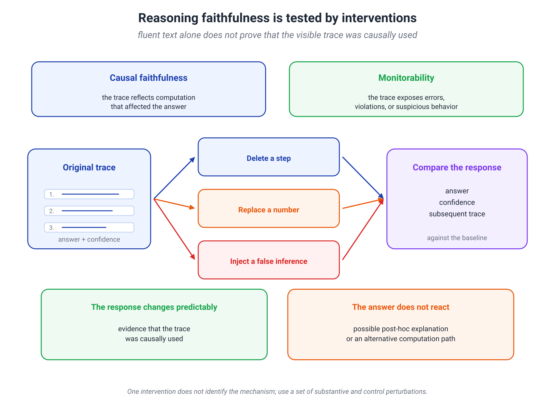
One way to test these properties is through interventions:
- remove a step;
- replace an intermediate number;
- insert a false conclusion;
- paraphrase the explanation without changing its content;
- hide part of the context referenced by the chain.
If the answer does not react to a materially important change, the chain may be a post-hoc explanation—or the system may have reconstructed the solution by another route. A single intervention rarely settles the question. We need controlled tasks, several intervention types, and comparison with external checks.
Recent work also shows that direct optimization pressure against a chain-of-thought monitor can reduce the chain’s diagnostic value: a system may learn to conceal the undesirable intent while retaining the behavior. This does not make chain monitoring useless. The narrower and more accurate conclusion is that monitorability is a separate system property that must be measured rather than assumed from high task accuracy.
13.6. One long trajectory or many candidates?
An extra budget can be spent in different ways. We can deepen one trajectory, generate many independent solutions, or build a tree with intermediate evaluation. The best choice depends on the error structure.
Voting over several trajectories
Suppose each independent attempt is correct with probability . For odd , the probability that a majority is correct is
If and the errors are genuinely independent, the majority becomes increasingly reliable. If , voting amplifies the systematic error.
Self-consistency applies a related idea: sample diverse reasoning paths and choose the most frequent final answer. Empirically, this can improve many multistep tasks. Independence, however, is a strong assumption. If every trajectory repeats the same mistaken template, the effective number of independent attempts remains close to one.
Best-of- with an ideal verifier
Suppose each candidate is correct with probability , and an ideal verifier recognizes correctness. The procedure succeeds whenever at least one of candidates is correct:
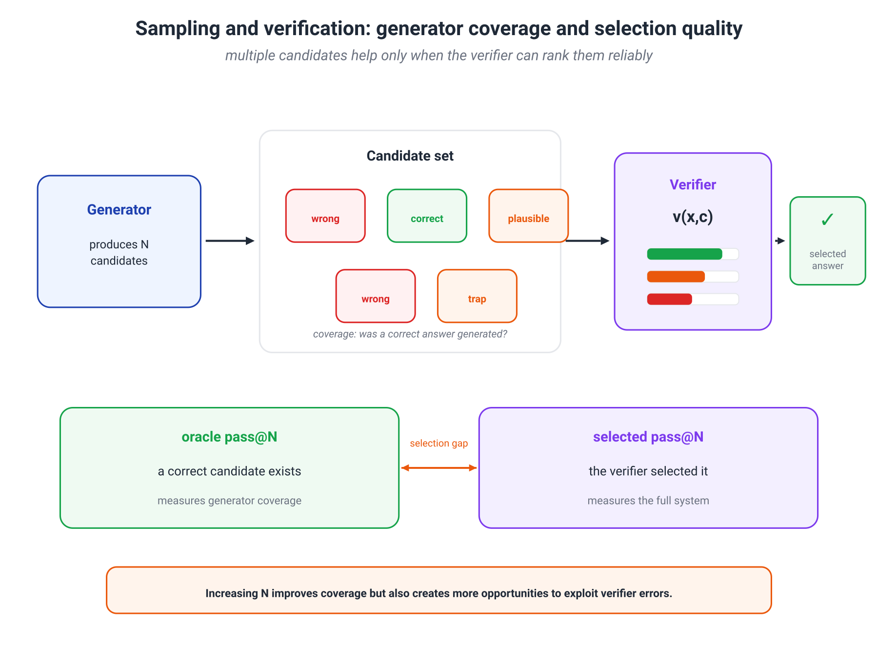
This formula measures generator coverage: did the search produce a valid answer at all?
An imperfect verifier
A real verifier assigns a score and selects the maximum. The outcome now depends on two components:
- the generator must include a correct answer;
- the verifier must rank it above the incorrect ones.
As increases, the first component improves while the second may deteriorate. A larger sample contains more correct solutions, but also more rare incorrect candidates that exploit a weakness of the scorer.
It is therefore useful to report two quantities:
- oracle pass@N: was a correct candidate present?
- selected pass@N: did the actual verifier select it?
Their gap measures the cost of imperfect selection.
Verification may be easier than construction—but not always
Some outputs are cheap to check: run the program on tests, substitute a root into an equation, or ask a proof assistant to verify a certificate. Broad search is particularly useful in such settings.
There is no universal theorem here that verification is always easier than generation. Tests may be incomplete, specifications ambiguous, and evaluating open-ended text nearly as difficult as producing it. Complexity-theoretic analogies can be suggestive, but they do not replace analysis of the actual verifier.
13.7. In-context learning: when context really brings evidence
Intermediate chains and prompt demonstrations are both text inside the context window, but their information roles differ.
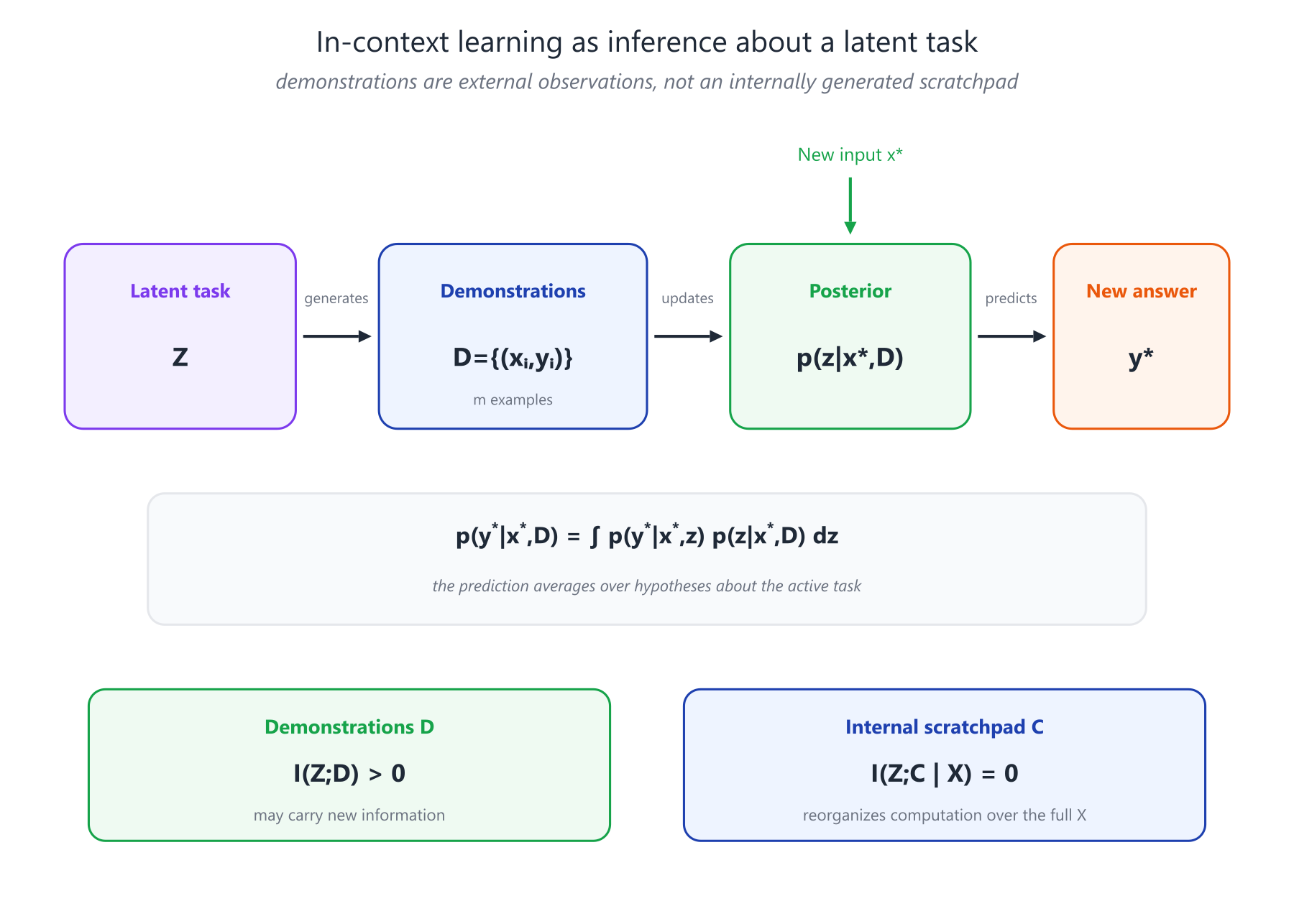
Let be a latent task, labeling convention, or rule, and let demonstrations
be conditionally independent given , each with law . Then
Let the new pair be conditionally independent of given , with the same law. The new input may also carry evidence about the task, so the prediction is
Here . If the new input is uninformative about given , the posterior simplifies to . This condition must be stated rather than assumed for arbitrary .
If the demonstrations depend on the latent task, then
They genuinely inform the system about the rule currently in force. An internal scratchpad constructed after the full prompt has been observed plays a different role: it organizes computation over the available context.
In special generative settings, in-context learning can be derived as implicit Bayesian inference over a latent concept. One such result is proved for mixtures of hidden Markov models under a specified structure for pretraining documents. Work on induction heads supplies another mechanistic picture for copying and continuing patterns.
The boundary matters. These special models do not imply that an arbitrary LLM explicitly stores an exact posterior, that every prompt was generated from a task mixture, or that all ICL behavior is Bayes-optimal. The latent-task model still supplies a useful question: which variable became better identified after the demonstrations, and which observations changed the state of knowledge?
13.8. How reasoning models are trained
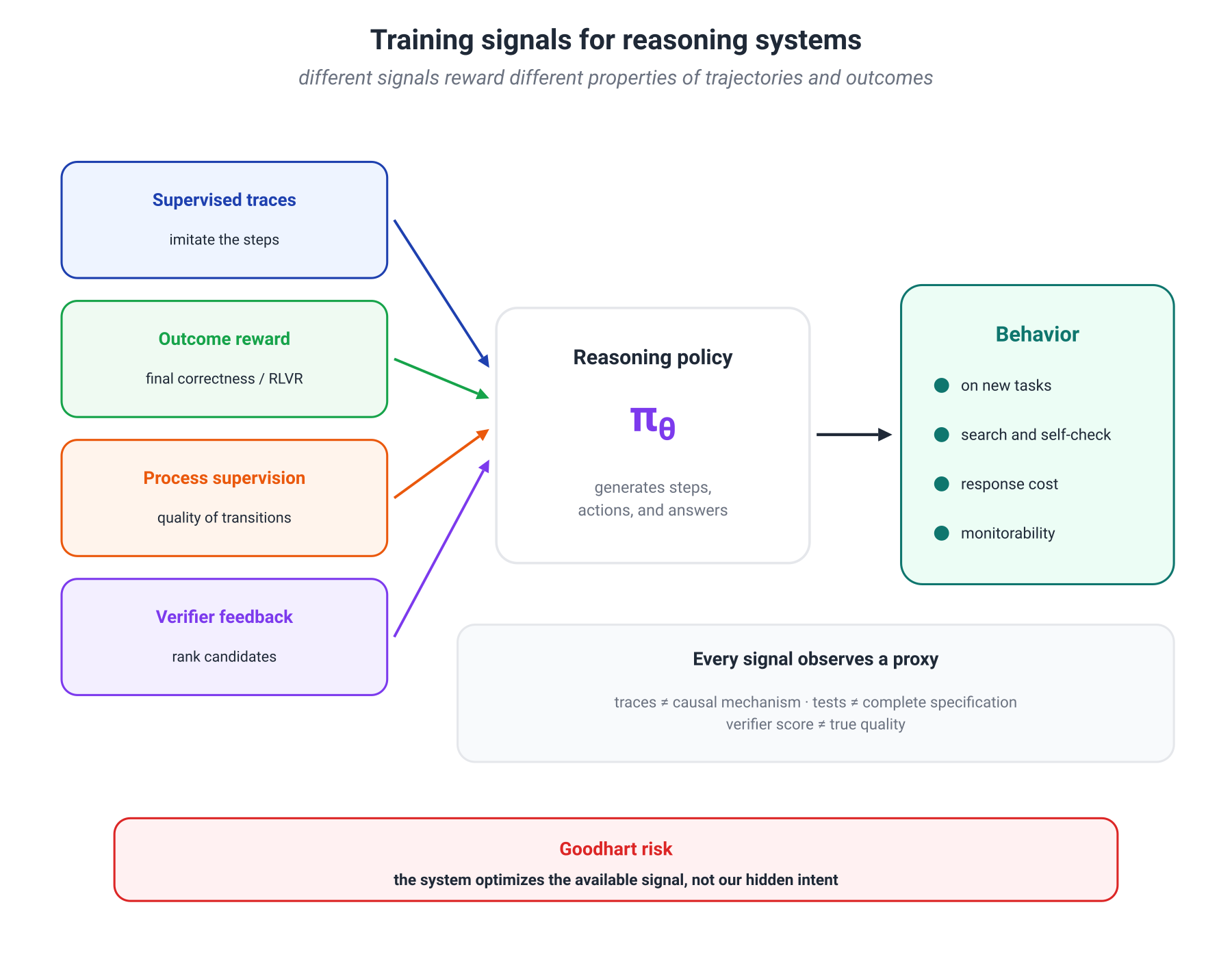
Modern multistep capabilities are often produced by several interacting loops. It is useful to separate imitation, generate-and-filter procedures, and optimization from feedback.
1. Imitating good trajectories
In supervised training, the model sees pairs of tasks and worked solutions and maximizes their likelihood. This teaches format, common decompositions, and local transitions.
The signal is dense, but it inherits the quality of the demonstrations. The model may learn unnecessary rituals, brittle shortcuts, or convincingly written mistakes.
2. Generate, verify, and train again
A common loop is:
- generate several trajectories;
- check final answers or intermediate steps;
- retain successful examples;
- fine-tune on the filtered data;
- repeat.
STaR is an early example of this bootstrapping pattern: the model generates rationales, keeps those that lead to correct answers, and learns from them. Rejection sampling, distillation, and synthetic reasoning datasets use related mechanics.
A systematic risk follows immediately: filtering can only reward what it can verify. If the check observes only the final answer, trajectories with incorrect intermediate reasons and accidentally correct outcomes may enter the training set.
3. Outcome and process feedback
Outcome rewards evaluate the end result: did the tests pass, did the numerical answer match, or was a formal condition satisfied? This signal scales well in domains with cheap automatic verification and underlies reinforcement learning with verifiable rewards (RLVR).
Process supervision evaluates intermediate transitions. It can localize errors and train a process reward model, but requires more expensive labels or a reliable automated checker.
Work on mathematical verifiers and stepwise supervision shows that selecting among candidates and supervising intermediate steps can substantially improve performance in their respective settings. DeepSeek-R1, meanwhile, demonstrated that large-scale reinforcement learning from verifiable outcomes can elicit long strategies of checking and revision; its full training pipeline then used additional stages, among other reasons, to improve readability and stable behavior.
Where Goodhart enters
Once a score becomes an optimization target, the system searches for ways to increase that score. Failure modes include:
- exploiting a weak verifier;
- passing incomplete tests;
- producing long but empty chains;
- imitating the style of a correct derivation without reliable substance;
- hiding undesirable behavior from a monitor.
KL regularization toward a reference policy can limit distributional drift, as discussed in Module 8. It is not a PAC-Bayes certificate and does not guarantee a truthful trajectory: the random objects, averaging operations, and theorem assumptions are different.
A useful engineering principle is:
The generator, verifier, and reward source form one system. No component can be evaluated independently of the errors made by the other two.
13.9. How to evaluate a reasoning system
A single final accuracy number hides too much. Two systems may reach the same score while one uses ten times more tokens. A generator may almost always include the answer while its verifier repeatedly selects the wrong candidate. A visible chain may help monitoring while poorly representing the causal computation.
We need a quality–cost frontier.
Answer quality
pass@1andpass@k;- accuracy after verifier selection;
- log loss and calibration when probabilities are available;
- robustness to paraphrases, changed numbers, and counterfactual variants.
Computational cost
- number of intermediate tokens;
- number of trajectories;
- FLOPs, latency, and monetary cost;
- number of tool calls;
- peak memory and allowed parallelism.
Search coverage and selection quality
- oracle pass@N;
- selected pass@N;
- error correlation across trajectories;
- verifier calibration and robustness;
- the budget beyond which additional sampling ceases to pay off.
Faithfulness and monitorability
- answer sensitivity to interventions on the chain;
- ability to localize the first erroneous step;
- agreement with formal checks;
- ability of an independent monitor to detect known violations;
- whether that ability survives optimization against the monitor.
Generalization
- new task templates rather than only new numbers;
- protection against benchmark contamination;
- transfer to different lengths and difficulty levels;
- domains with weaker automatic verification;
- agent settings under distribution shift.
Adaptive budgets
Let denote quality under compute budget . We care not only about the highest point but about the shape of the curve:
Easy prompts may be solved almost immediately. Medium-difficulty prompts may benefit from several samples or a longer trajectory. For tasks beyond the current model’s coverage, extra compute may only produce many variants of the same error.
A study of compute-optimal test-time scaling found that the best way to spend inference compute depends strongly on prompt difficulty. In its setting, adaptive allocation was more than four times as efficient as a best-of- baseline; on a subset of tasks, a smaller model with extra inference compute outperformed a model with fourteen times as many parameters at matched FLOPs.
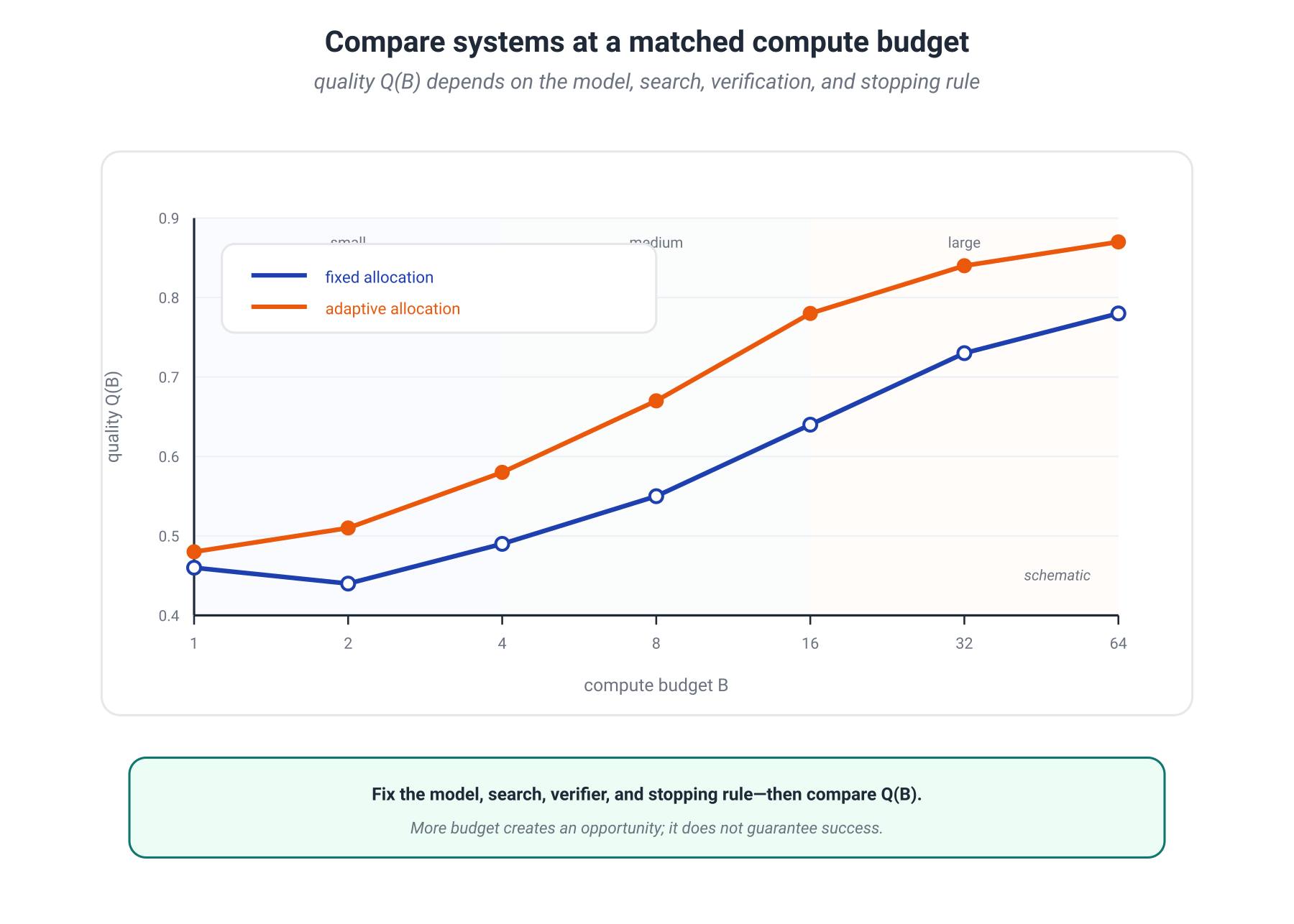
This is not a law that inference compute always beats model scaling. The result requires nonzero generator coverage, a useful verifier, and an appropriate budget allocation rule. A fair comparison therefore fixes the full search, verification, and stopping protocol—not only the base model.
13.10. What is proved, what is observed, and what remains a hypothesis
Reasoning research makes it especially easy for a useful image to turn into an alleged law. We therefore classify the claims by status.
Exact results within stated models
- If an internal chain is generated only from the complete input and independent randomness, then
- Under independent attempts, majority accuracy has the binomial form above.
- With an ideal verifier,
- Demonstrations can carry information about a latent task.
- Under special assumptions, sequential CoT steps increase Transformer computational expressivity.
Empirical findings
- Step-by-step prompting improves a range of multistep tasks.
- Additional test-time compute can yield large gains, but the gain depends on task and strategy.
- Verifiers and process supervision are useful in some domains with checkable outcomes.
- Visible chains are not always faithful reports of the causal mechanism.
- Chains can support monitoring, but that value is sensitive to optimization pressure.
Research lenses
- reasoning as a trade-off between amortization and search;
- trajectory length as a proxy for computational difficulty;
- stepwise information gain as a universal measure of reasoning quality;
- an LLM as a finite approximation to a universal predictor.
The final group is valuable when it leads to a testable model. It becomes dangerous when the domain of the analogy disappears from the claim.
13.11. Mathematical deepening: stepwise information gain
Optional on a first pass. We now state when a reduction in cross-entropy can be related to conditional mutual information and why the definition of the state changes the interpretation.
Arbitrary and nested states
For arbitrary and ,
Subtracting gives the exact identity
Thus the reduction in conditional entropy between two arbitrary states is a net balance: newly available relevant information minus relevant information lost when the old state is replaced.
If the old state can be recovered from the new one, then
and we obtain
The nesting condition cannot be silently omitted.
An internal step followed by an external observation
Suppose that at step the system first constructs an internal state and then receives an external observation . Let
be the full history. If is generated from and independent randomness, then
By the chain rule,
In the complete information accounting, the new signal arrived through . The internal step may determine which observation to request, thereby making the observation more valuable, but it did not itself create an external fact.
Cross-entropy of an auxiliary predictor
Let predict the answer from state . Its expected cross-entropy is
It decomposes as
where
is the variational gap.
For arbitrary states,
A cross-entropy difference equals conditional mutual information only under two additional conditions:
- the old state is recoverable from the new one;
- the predictor gaps are equal, negligible, or separately controlled.
The predictive entropy of one model does not establish either condition.
Why a working state can become “more informative”
A subtle point remains. If the state update is
and receives neither nor external data, the data-processing inequality gives
Information cannot increase.
In an LLM, however, each step typically attends to the original prompt again:
A compressed working state can therefore have greater mutual information with than : it has extracted another relevant aspect of . The complete pair , however, still carries no more information about than alone.
This is the correct distinction:
- accessibility to a restricted state or readout may increase;
- the total information in the complete input plus internal chain does not increase without an external observation.
Sequential expressivity
Information theory asks where the evidence came from. Computational theory asks which functions can be implemented under a budget.
Under particular assumptions on precision and representation size, a fixed-depth Transformer without CoT is restricted to a class of parallel computations, while sequential steps can realize circuits of size on the order of . The two languages therefore complement one another:
- mutual information accounts for available evidence;
- computational expressivity accounts for the ability to transform that evidence into an answer.
13.13. Conclusion: information is not computation
The course began by separating information from meaning. It ends with a related but new distinction: information and computation are not the same thing.
A system may receive all the necessary data and still fail to compute the answer. It may correctly transform known data without learning a new fact. It may retrieve new evidence but integrate it poorly. And it may produce a persuasive explanation that only partially reflects the causal mechanism behind the answer.
A reasoning system should therefore be analyzed along several axes:
- parameters provide amortized competence;
- intermediate tokens provide sequential depth and working memory;
- candidate sampling provides search breadth;
- a verifier provides a selection rule;
- tools and environments may provide either computation or new observations;
- the metric defines what the system is trained to count as success.
Information theory plays its best role here. It does not promise a magical definition of intelligence; it forces us to identify random variables, data sources, conditional dependencies, and error costs. Computational theory adds the question of which procedures are available. Experimental methodology asks whether the proposed mechanism survives beyond one benchmark.
Extra tokens are not automatically extra knowledge. More often, they provide extra time, working memory, search breadth, and opportunities for checking.
This separation lets us discuss modern reasoning systems without either extreme: reducing them to “just the next token,” or treating a long chain as proof of understanding.
Primary sources
- J. Wei et al., Chain-of-Thought Prompting Elicits Reasoning in Large Language Models, 2022.
- X. Wang et al., Self-Consistency Improves Chain of Thought Reasoning in Language Models, 2022.
- K. Cobbe et al., Training Verifiers to Solve Math Word Problems, 2021.
- S. Yao et al., Tree of Thoughts: Deliberate Problem Solving with Large Language Models, 2023.
- H. Lightman et al., Let’s Verify Step by Step, 2023.
- C. Snell et al., Scaling LLM Test-Time Compute Optimally can be More Effective than Scaling Model Parameters, 2024.
- J.-F. Ton, M. F. Taufiq, Y. Liu, Understanding Chain-of-Thought in LLMs through Information Theory, 2024.
- T. Lanham et al., Measuring Faithfulness in Chain-of-Thought Reasoning, 2023.
- Y. Chen et al., Reasoning Models Don’t Always Say What They Think, 2025.
- B. Baker et al., Monitoring Reasoning Models for Misbehavior and the Risks of Promoting Obfuscation, 2025.
- Z. Li et al., Chain of Thought Empowers Transformers to Solve Inherently Serial Problems, 2024.
- S. M. Xie et al., An Explanation of In-context Learning as Implicit Bayesian Inference, 2021.
- C. Olsson et al., In-context Learning and Induction Heads, 2022.
- E. Zelikman et al., STaR: Bootstrapping Reasoning With Reasoning, 2022.
- DeepSeek-AI, DeepSeek-R1: Incentivizing Reasoning Capability in LLMs via Reinforcement Learning, 2025.