Module 3. Cross-Entropy and KL Divergence

How to read this module. Sections 3.1–3.7 form the main route. We begin with log-loss, separate uncertainty in the data from model mismatch, carry the decomposition into classification and language modeling, and end with the logit gradient and perplexity. Section 3.8 is a mathematical deepening on KL direction under a restricted model family. Section 3.9 is a map of applications; read it selectively and return to it as variational inference, distillation, and RLHF become relevant.

3.1. The model returns a distribution; the world returns one outcome

A probabilistic model rarely answers with a single class. It returns a distribution. Taking the argmax keeps the winner and discards most of the information.

Consider two three-class classifiers:

$$q_A=(0.55,0.40,0.05), \qquad q_B=(0.95,0.04,0.01).$$

Both choose the first class. If that class is observed, model $B$ receives a much better logarithmic score:

$$-\ln 0.55\approx0.598, \qquad -\ln 0.95\approx0.051.$$

But if the second class is correct, the picture reverses:

$$-\ln 0.40\approx0.916, \qquad -\ln 0.04\approx3.219.$$

Confidence is valuable when it points in the right direction and expensive when the model is confidently wrong. This is exactly what logarithmic loss (log-loss) measures. For an observed outcome $y$,

$$\ell(q,y)=-\log q(y).$$

The logarithm does two jobs at once. It turns the product of sequence probabilities into a sum of token losses, and it strongly penalizes a model that declared an observed event nearly impossible.

We now introduce the two roles that run through the module:

• $P$ is the distribution generating the data;
• $Q_\theta$ is a probabilistic model with parameters $\theta$.

In classification these are conditional distributions

$p(y\mid x),\qquad q_\theta(y\mid x),$

and in an autoregressive language model,

$p(x_t\mid x_{<t}),\qquad q_\theta(x_t\mid x_{<t}).$

We do not receive $P$ as a ready-made table. We observe individual outcomes from $P$ and ask, each time: how much probability did the model assign to what actually happened? Averaging those scores leads to cross-entropy.

Module 2 used entropy to quantify the uncertainty of one distribution. We now have two distributions, and the engineering question becomes: how much of the average loss is unavoidable uncertainty in the data, and how much comes from the model failing to match them?

Unless stated otherwise, the alphabet on the main route is finite. We write the logarithm base as $b$: $b=2$ gives bits and $b=e$ gives nats. Deep-learning libraries normally use the natural logarithm, so training losses are usually reported in nats.

The historical line has two steps. Shannon tied $-\log p$ to the information length of a message; Kullback and Leibler formalized a directed discrepancy between two distributions. Modern cross-entropy training joins those ideas.

3.2. Cross-entropy: the model's average logarithmic bill

For distributions $P=(p(x))$ and $Q=(q(x))$ on the same alphabet, cross-entropy is

$$\boxed{ H_b(P,Q) =\mathbb E_{X\sim P}[-\log_b q(X)] =-\sum_x p(x)\log_b q(x) }.$$

Read the formula by role:

• the first argument $P$ says where outcomes come from and what distribution defines the average;
• the second argument $Q$ says whose probabilities appear inside the logarithm.

Cross-entropy is therefore directed:

$H(P,Q)\ne H(Q,P)$

in general. Swapping the arguments changes the experiment: it changes both the source of events and the model being scored.

From individual losses to an expectation

If $x_1,\ldots,x_N$ are observations from $P$, the sample average

$$\widehat L_b(Q) =-\frac1N\sum_{i=1}^N\log_b q(x_i)$$

estimates $H_b(P,Q)$. Under standard conditions, the law of large numbers turns the sample average into the population expectation. That is why a training loop can work one example at a time even though the formal statement about model quality lives at the distribution level.

For conditional prediction—classification, probabilistic regression, or next-token prediction—the natural quantity is

$$H_P(Y\mid C;Q) :=\mathbb E_{(C,Y)\sim P}[-\log q(Y\mid C)].$$

The semicolon separates the data distribution $P$ from the predictor $Q$ being evaluated. Below we usually call this simply conditional cross-entropy.

One label is one observation, not the entire conditional law

In supervised learning, a target label $y$ is often represented by a one-hot vector $e_y$. The per-example loss is then

$$-\sum_{k=1}^K(e_y)_k\log q_k=-\log q_y.$$

This is a convenient representation of the observed event. It does not turn the true $P(Y\mid X=x)$ into a degenerate one-hot law. The same input may admit ambiguous annotation, several valid continuations, label noise, or hidden context. A dataset reveals one outcome at a time; the distribution emerges through repetition and structure.

When the model calls a possible event impossible

Two boundary conventions matter. An outcome with zero mass under $P$ contributes nothing:

$0\log\frac{0}{q}:=0.$

But if $p(x)>0$ and $q(x)=0$, then

$-p(x)\log q(x)=+\infty.$

The model assigned zero probability to an event that occurs, so its average logarithmic bill is infinite. Finiteness is written as $P\ll Q$: the support of $P$ must lie inside the support of $Q$.

With finite logits, a softmax network assigns formally positive probability to every class. Numerically, however, very small values may underflow to zero. Cross-entropy is therefore computed through a stable log_softmax form rather than by applying softmax and log as separate operations.

3.3. KL divergence: the part of the loss attributable to the model

The entropy of the source is

$H_b(P)=-\sum_x p(x)\log_b p(x).$

Add and subtract $\log_b p(x)$ inside the cross-entropy:

$$\begin{aligned} H_b(P,Q) &=-\sum_x p(x)\log_b q(x)\\ &=-\sum_x p(x)\log_b p(x) +\sum_x p(x)\log_b\frac{p(x)}{q(x)}. \end{aligned}$$

The second term is the KL divergence, or relative entropy:

$$D_{\mathrm{KL},b}(P\|Q) :=\sum_x p(x)\log_b\frac{p(x)}{q(x)}.$$

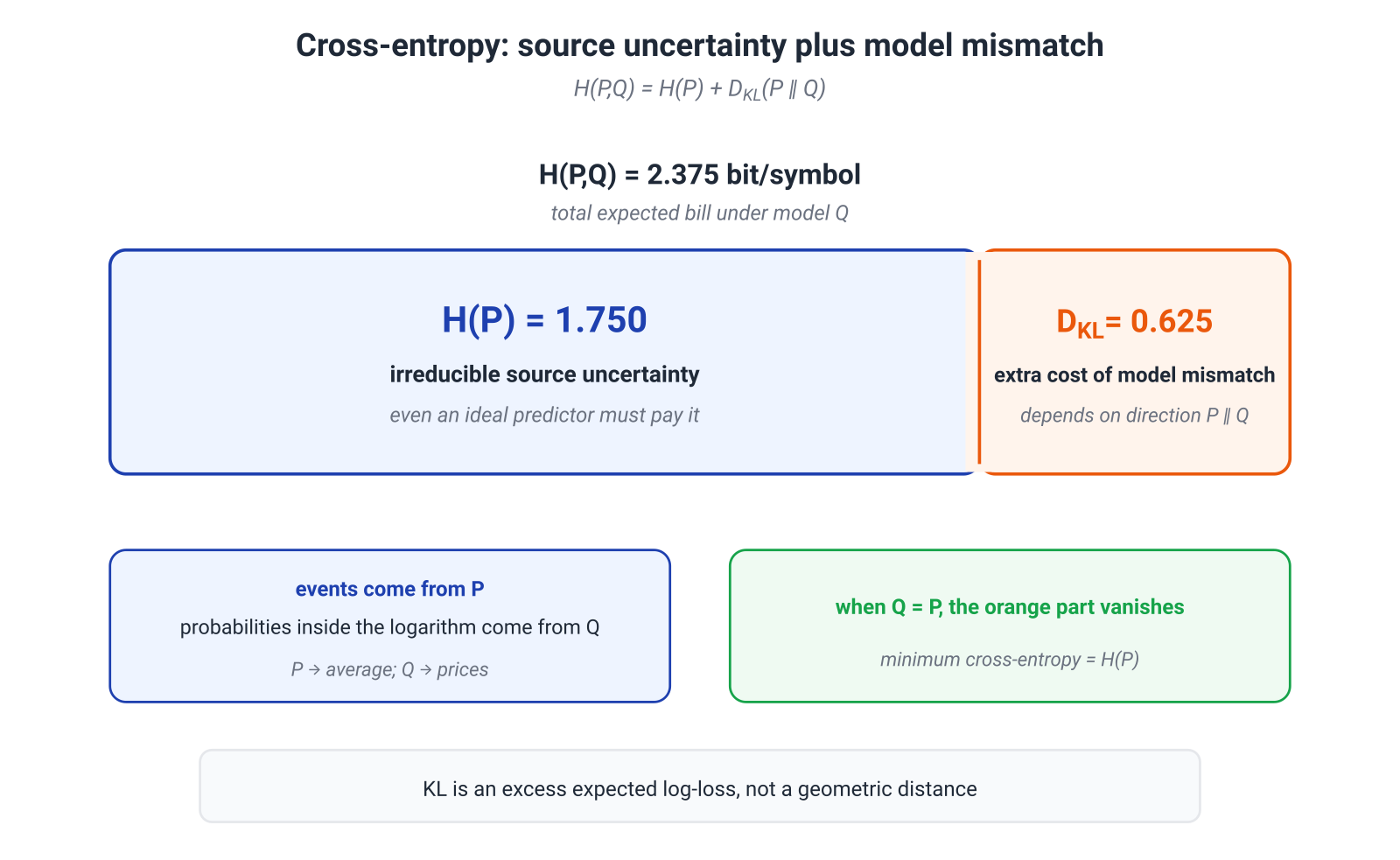
This gives the central identity of the module:

$$\boxed{ H_b(P,Q)=H_b(P)+D_{\mathrm{KL},b}(P\|Q) }.$$

Read the decomposition in words.

• $H(P)$ is the uncertainty that remains even for an ideal predictor that knows $P$;
• $D_{\mathrm{KL}}(P\|Q)$ is the extra bill caused by the mismatch between model $Q$ and data distribution $P$.

A useful compact formulation is:

KL is the average surcharge for using the wrong probabilistic model.

KL is not a metric: it is asymmetric and need not satisfy the triangle inequality. For optimization, that is not a defect. The problem itself is directed: outcomes come from $P$, while probabilities are supplied by $Q$.

Why the surcharge is non-negative

If some $x$ has $p(x)>0$ and $q(x)=0$, the KL divergence is $+\infty$. Otherwise, let

$\mathcal S=\{x:p(x)>0\}$

be the positive support and use $\ln u\le u-1$:

$$\begin{aligned} -D_{\mathrm{KL}}(P\|Q) &=\sum_{x\in\mathcal S}p(x) \ln\frac{q(x)}{p(x)}\\ &\le\sum_{x\in\mathcal S}p(x) \left(\frac{q(x)}{p(x)}-1\right)\\ &=\sum_{x\in\mathcal S}q(x)-1\\ &\le0. \end{aligned}$$

Hence

$D_{\mathrm{KL}}(P\|Q)\ge0.$

Equality requires both $q(x)=p(x)$ on $\mathcal S$ and no $Q$-mass outside $\mathcal S$. Therefore,

$$D_{\mathrm{KL}}(P\|Q)=0 \quad\Longleftrightarrow\quad P=Q.$$

This is Gibbs' inequality. Module 4 will recover the same result from Jensen's inequality and the log-sum inequality. The mechanism matters here: average log-loss splits into an unavoidable term and a non-negative model error.

Log-loss asks for the full distribution

The decomposition immediately gives

$$\mathbb E_{Y\sim P}[-\log q(Y)] \ge \mathbb E_{Y\sim P}[-\log p(Y)],$$

with a unique minimum at $Q=P$. Log-loss is therefore a strictly proper scoring rule: in expectation, reporting the true distribution is optimal, not merely reporting the correct most likely class.

This is stronger than an argmax guarantee. Two predictors can have identical accuracy and different cross-entropy because one allocates probability more faithfully between the observed outcome and its alternatives. That is why log-loss is useful when probabilities, calibration, and downstream decisions under different error costs matter.

What maximum likelihood actually does

For a model $q_\theta$, maximizing likelihood is equivalent to minimizing empirical negative log-likelihood (NLL). At the population level the objective is

$$\min_\theta D_{\mathrm{KL}}(P\|Q_\theta),$$

because $H(P)$ does not depend on $\theta$.

If the model family contains $P$ and the usual statistical conditions hold, the population optimum is the true distribution. Under misspecification, the model chooses the best available KL projection:

$$\theta^*\in \arg\min_\theta D_{\mathrm{KL}}(P\|Q_\theta).$$

This does not weaken the meaning of maximum likelihood; it states it precisely. The objective says what approximation counts as best inside the chosen family. Finite data, sample quality, and optimization determine how closely a particular training run approaches that population solution.

3.4. The wrong code: how KL becomes extra bits

In bits, the quantity

$$\ell_Q(x)=-\log_2 q(x)$$

is the ideal information length of outcome $x$ under model $Q$. If actual symbols come from $P$, the average bill is

$$\mathbb E_P[\ell_Q(X)]=H_2(P,Q).$$

An ideal code matched to the source itself would have average information length $H_2(P)$. The difference is

$$H_2(P,Q)-H_2(P) =D_{\mathrm{KL},2}(P\|Q).$$

This gives KL an operational reading: the average number of extra bits paid when data from $P$ are encoded using probabilities from model $Q$.

A real binary prefix code needs integer lengths. The connection survives with a small overhead. A Shannon code built from $Q$ uses

$$L_Q(x)=\left\lceil-\log_2 q(x)\right\rceil,$$

so

$$H_2(P,Q) \le \mathbb E_P[L_Q(X)] < H_2(P,Q)+1.$$

For blocks of length $n$, the overhead is less than one bit per block, hence less than $1/n$ bit per symbol. Arithmetic and range coding implement this idea in practice. Thus “KL is extra bits” is not merely a metaphor; it is an asymptotic engineering statement.

A dyadic example: equal entropy, unequal mismatch cost

Let

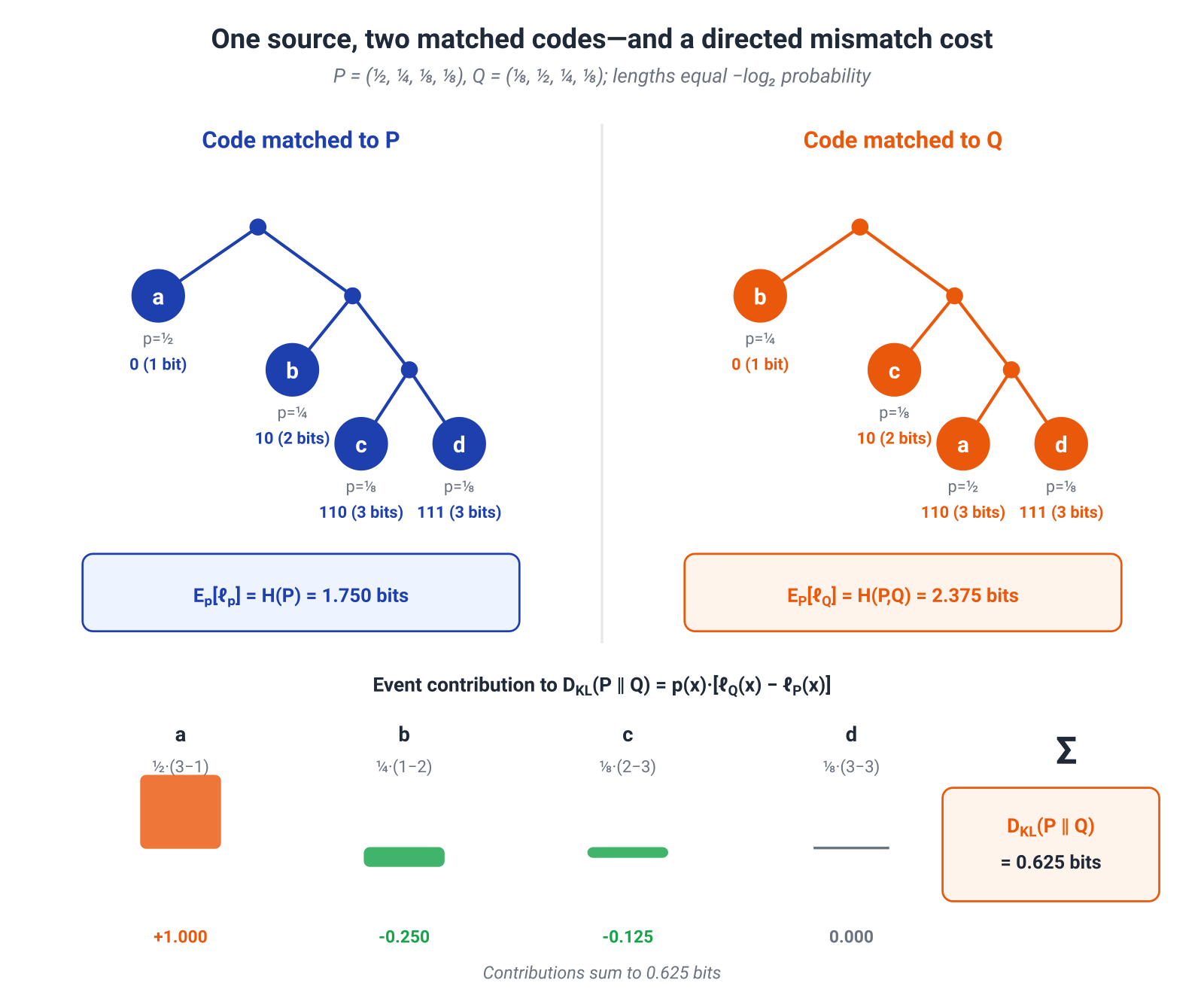
$$P=\left(\frac12,\frac14,\frac18,\frac18\right), \qquad Q=\left(\frac18,\frac12,\frac14,\frac18\right).$$

Both distributions are dyadic, so their ideal lengths are integers:

Their entropies are equal:

$H_2(P)=H_2(Q)=1.75\ \text{bits/symbol}.$

But the code matched to $Q$ is especially expensive for the most frequent event $x_1$, giving

$$H_2(P,Q)=2.375, \qquad D_{\mathrm{KL},2}(P\|Q)=0.625\ \text{bits}.$$

In the reverse direction,

$$H_2(Q,P)=2.25, \qquad D_{\mathrm{KL},2}(Q\|P)=0.5\ \text{bits}.$$

Equal entropy means that the two sources have equal average uncertainty. It does not mean that substituting one model for the other has equal cost. Direction determines which events occur often and what prices the mismatched code assigns to them.

3.5. One formula for classification and language modeling

Let $C$ be a context and $Y$ a label or next token. The expected conditional log-loss is

$$\mathcal L(\theta) =\mathbb E_{(C,Y)\sim P} [-\log q_\theta(Y\mid C)].$$

Apply the previous decomposition at each context and then average over $C$:

$$\boxed{ \mathcal L(\theta) =H_P(Y\mid C) +\mathbb E_{C\sim P} D_{\mathrm{KL}} \!\left( P(\cdot\mid C) \|Q_\theta(\cdot\mid C) \right) }.$$

The distinction between task uncertainty and model error is now explicit.

• $H_P(Y\mid C)$ is the ambiguity of the next outcome after the available context;
• the conditional KL is the average mismatch between the true and modeled continuation distributions.

If the same context admits several natural answers, even an ideal model need not achieve zero loss on every example. It should distribute probability correctly across valid continuations.

An autoregressive sequence

For a sequence of length $T$,

$$p(x_{1:T})=\prod_{t=1}^T p(x_t\mid x_{<t}), \qquad q_\theta(x_{1:T})=\prod_{t=1}^T q_\theta(x_t\mid x_{<t}).$$

The logarithm turns the product into a sum:

$$-\log q_\theta(x_{1:T}) =\sum_{t=1}^T- \log q_\theta(x_t\mid x_{<t}).$$

After averaging,

$$\mathbb E_P[-\log q_\theta(X_{1:T})] =H_P(X_{1:T}) +D_{\mathrm{KL}}(P_{1:T}\|Q_{\theta,1:T}).$$

The KL chain rule then decomposes the joint mismatch step by step:

$$\boxed{ D_{\mathrm{KL}}(P_{1:T}\|Q_{\theta,1:T}) = \sum_{t=1}^T \mathbb E_{X_{<t}\sim P} D_{\mathrm{KL}} \!\left( P(\cdot\mid X_{<t}) \|Q_\theta(\cdot\mid X_{<t}) \right) }.$$

This is the exact information-theoretic form of standard language-model training: every token sends the model a logarithmic bill, and total NLL adds those bills along the sequence.

Teacher forcing: score the model where the data live

Under teacher forcing, the context $X_{<t}$ comes from the data. This makes the objective tractable and directly evaluates the model's conditional probabilities on real prefixes. Those are precisely the prefixes weighting the KL terms above.

During free generation, the model gradually creates its own contexts. An early error changes the next input, then the next one, and the visited-prefix distribution may move from $P$ toward the distribution induced by $Q_\theta$. Validation NLL under teacher forcing therefore measures conditional modeling quality on the data distribution, but it does not replace a separate evaluation of behavior on the model's own trajectories.

This boundary is useful rather than discouraging. It suggests an evaluation design: held-out NLL tests probabilistic modeling of the data; generation tests, interactive scenarios, and robustness checks test behavior after the model has accumulated its own decisions.

What the next-token objective promises

At the population level, the objective rewards

$$Q_\theta(\cdot\mid C) \approx P(\cdot\mid C)$$

for contexts drawn from the data. That is a strong, precise statement. Factual correctness, useful abstention, and preference alignment arise to the extent that the data and task definition encode them. Retrieval, verification tools, preference fine-tuning, and specialized evaluation add signals that ordinary next-token NLL does not contain.

Low NLL is therefore a foundational property of a probabilistic language model, but not the only metric of a deployed system.

3.6. Why CrossEntropyLoss is so convenient to optimize

Let the network produce logits $z\in\mathbb R^K$, with probabilities

$$q_j =\operatorname{softmax}(z)_j =\frac{e^{z_j}}{\sum_k e^{z_k}}.$$

For a target distribution $r=(r_1,\ldots,r_K)$, where $r_j\ge0$ and $\sum_j r_j=1$, the cross-entropy loss is

$$\begin{aligned} \ell(z;r) &=-\sum_{j=1}^K r_j\log q_j\\ &=\log\sum_{k=1}^Ke^{z_k} -\sum_{j=1}^K r_jz_j. \end{aligned}$$

This form exposes the optimization structure: logsumexp accounts for all classes, while the second term raises logits according to the target distribution.

Differentiation gives one of the most useful formulas in deep learning:

$$\boxed{ \frac{\partial\ell}{\partial z_j}=q_j-r_j }.$$

For a one-hot target $r=e_y$,

$$\nabla_z\ell=q-e_y.$$

The model lowers logits for classes to which it assigned more probability than the target requires and raises the observed class logit. The update is already scaled by the current probabilities; no separate hand-designed softmax factor is needed.

The Hessian is

$$\nabla_z^2\ell =\operatorname{diag}(q)-qq^\top.$$

For every vector $v$,

$$\begin{aligned} v^\top\nabla_z^2\ell\,v &=\sum_j q_jv_j^2 -\left(\sum_j q_jv_j\right)^2\\ &=\operatorname{Var}_{J\sim q}(v_J)\ge0. \end{aligned}$$

Cross-entropy is therefore convex in the logits. A deep network is still non-convex in its weights because the logits are a nonlinear function of many layers of parameters.

The numerically stable form

Computing softmax and then log separately is unsafe: exponentials of large logits may overflow, while tiny probabilities may underflow to zero. Use

$$\log\sum_k e^{z_k} =m+\log\sum_ke^{z_k-m}, \qquad m=\max_kz_k.$$

Accordingly, PyTorch's nn.CrossEntropyLoss and F.cross_entropy expect raw, unnormalized logits. With class-index targets, the fused operation corresponds to log_softmax followed by NLL:

import torch
import torch.nn.functional as F

logits = torch.tensor([[2.0, -1.0, 0.5]], requires_grad=True)
target = torch.tensor([2])

loss_fused = F.cross_entropy(logits, target)
loss_manual = F.nll_loss(F.log_softmax(logits, dim=-1), target)

assert torch.allclose(loss_fused, loss_manual)
loss_fused.backward()

The fused implementation is not only faster; it preserves the correct numerical scale of the computation.

One API can define several statistical objectives

With label smoothing, the one-hot target is replaced, for example, by

$$r=(1-\varepsilon)e_y+\varepsilon u,$$

where $u$ is a smoothing distribution, often uniform. The logit gradient remains $q-r$, but the population optimum now corresponds to the smoothed conditional distribution. This is a deliberate regularizer rather than ordinary NLL on the original one-hot observations.

Class weights change the relative cost of errors. ignore_index, masking, and the reduction mode determine which elements enter the average and with what normalization. The name CrossEntropyLoss therefore does not fully specify the statistical risk: targets, weights, masks, and normalization matter.

Token perplexity is normally computed from an unsmoothed, unweighted mean NLL over exactly the target tokens included by the evaluation protocol.

3.7. Perplexity: returning from the logarithmic scale

NLL is convenient for addition and optimization, but its logarithmic scale is not always intuitive. Perplexity (PPL) exponentiates the average loss back to a multiplicative scale.

For $N$ observed targets,

$$\widehat L_b =-\frac1N\sum_{i=1}^N\log_b q_i(y_i),$$

and

$$\boxed{ \operatorname{PPL}=b^{\widehat L_b} }.$$

If NLL is measured in nats,

$\operatorname{PPL}=e^{\widehat L},$

while in bits,

$\operatorname{PPL}=2^{\widehat L_2}.$

The equivalent form is especially informative:

$$\operatorname{PPL} = \left( \prod_{i=1}^N\frac1{q_i(y_i)} \right)^{1/N}.$$

PPL is therefore the geometric mean reciprocal probability assigned to the observed targets.

A small example

Suppose the model assigns the observed tokens probabilities

$\frac12,\qquad\frac14,\qquad\frac18.$

The mean NLL in bits is

$$\widehat L_2=\frac{1+2+3}{3}=2,$$

so

$$\operatorname{PPL}=2^2=4.$$

The same result follows from the geometric mean:

$$(2\cdot4\cdot8)^{1/3}=4.$$

The phrase “effective number of equally likely choices” is exact when the model really is uniform over the same number of outcomes at every step. For a general distribution it is a useful scale, not a literal count of candidates.

PPL and predictive entropy answer different questions

The model's predictive entropy at context $c$ is

$$H(Q_\theta(\cdot\mid c)) =-\sum_yq_\theta(y\mid c)\log q_\theta(y\mid c).$$

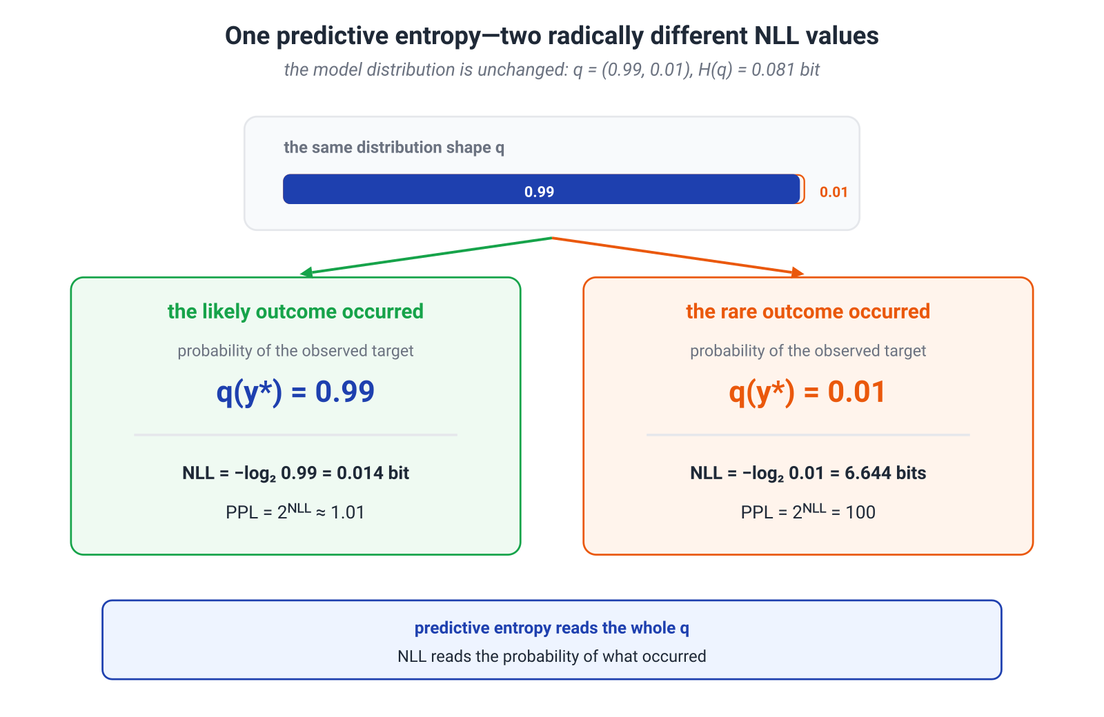
It measures how spread out the model's own distribution is. NLL and PPL look at the probability of the realized outcome.

A confident model can therefore have very low predictive entropy and enormous PPL if it is confident in the wrong answer. Conversely, an objectively ambiguous context can have high entropy and good expected NLL when probability mass is allocated correctly across valid continuations.

At the population level, the decomposition from Section 3.5 gives

$$\mathcal L(\theta)\ge H_P(Y\mid C),$$

with equality for an ideal conditional predictor. The minimum inside a restricted family may be higher. A finite validation estimate is random and can occasionally fall below its expectation, so a single validation number or extrapolated scaling-law asymptote should not automatically be called the “true entropy of language.”

Comparing perplexities

PPL depends on what counts as a prediction event. Different tokenizers split the same string into different numbers of tokens, so token-level perplexities cannot be compared directly across tokenizers.

A sound comparison requires at least:

• the same corpus and preprocessing;
• the same tokenizer;
• the same context length and context policy;
• the same target mask and normalization.

Bits per byte or per character provide a common physical unit and improve comparability, although corpus composition and the context protocol remain part of the experiment. Module 6 will make this connection literal: a probabilistic model becomes a compressor, and NLL becomes a measurable file length.

3.8. Mathematical deepening: why KL direction changes the answer

Optional on a first pass. For the main route, it is enough to know that maximum likelihood minimizes $D(P\|Q)$ and that direction matters most when the model family cannot represent the target distribution exactly.

We now move from sums to densities:

$$D_{\mathrm{KL}}(P\|Q) =\int p(x)\log\frac{p(x)}{q(x)}\,dx.$$

In this section we call

$D_{\mathrm{KL}}(P\|Q)$

forward KL from target $P$ to approximation $Q$, and

$D_{\mathrm{KL}}(Q\|P)$

reverse KL. The terminology depends on which distribution is designated as the target, so the argument order is always more important than the label.

The two directions average in different places:

• forward KL takes an expectation under $P$: every region containing data gets a vote;
• reverse KL takes an expectation under $Q$: the model pays mainly for regions where it places its own mass.

If all distributions are allowed and $P$ is exactly representable, both directions share the minimum $Q=P$. The difference becomes visible under model misspecification.

Canonical example: two peaks and one Gaussian

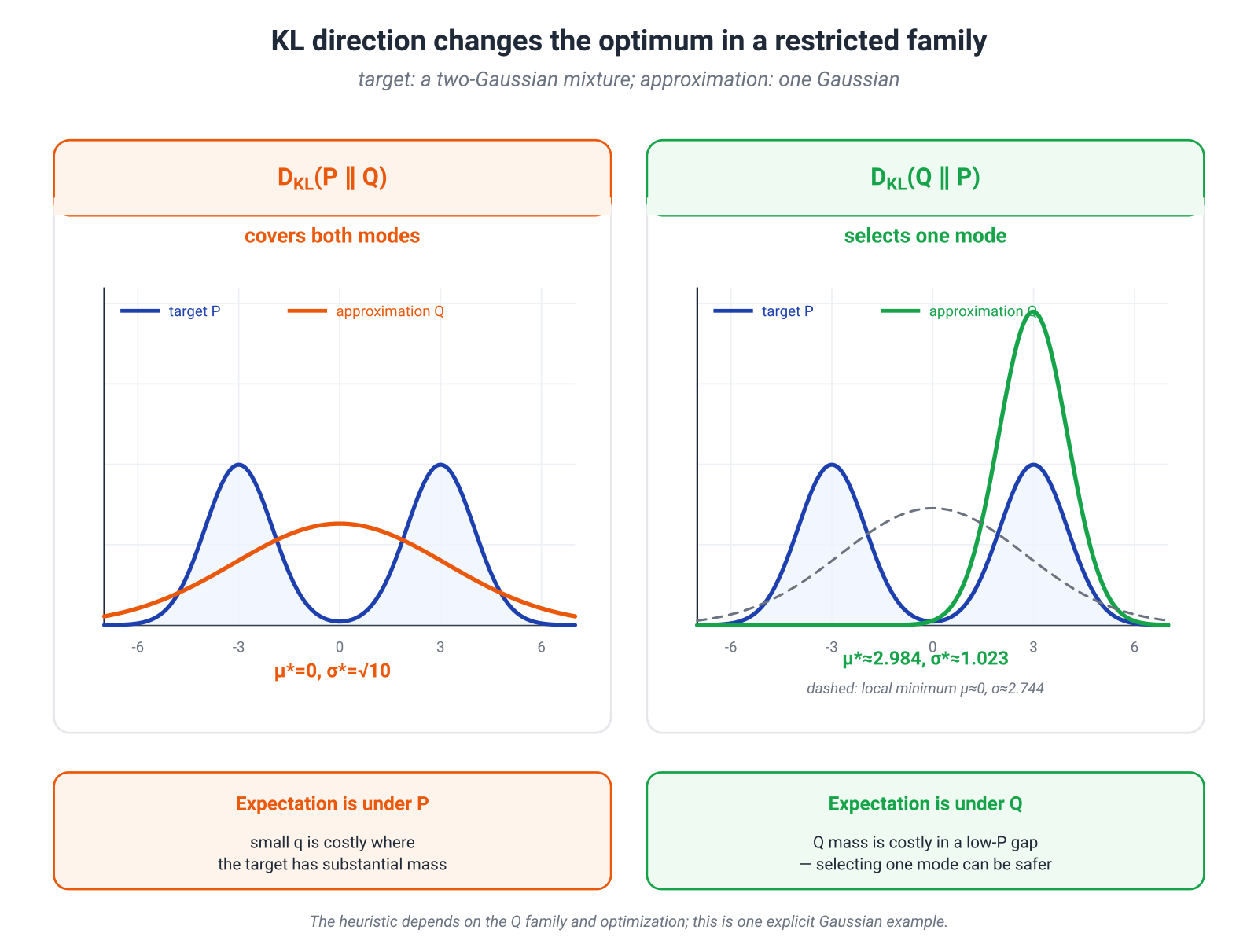
Let the target density be

$$p(x) =\tfrac12\mathcal N(x;-3,1) +\tfrac12\mathcal N(x;3,1),$$

while the model is restricted to a single Gaussian

$q_{\mu,\sigma}(x)=\mathcal N(x;\mu,\sigma^2).$

Forward KL: both peaks must be explained

For fixed $P$, minimizing $D(P\|Q_{\mu,\sigma})$ is equivalent to minimizing

$$-\mathbb E_P[\log q_{\mu,\sigma}(X)] = \frac12\log(2\pi\sigma^2) + \frac{\mathbb E_P[(X-\mu)^2]}{2\sigma^2}.$$

The optimal Gaussian matches the mean and variance of $P$:

$$\mu^*=\mathbb E_P[X]=0, \qquad (\sigma^*)^2=\operatorname{Var}_P(X)=1+3^2=10.$$

Thus

$$\mu^*=0, \qquad \sigma^*=\sqrt{10}\approx3.162.$$

The model covers both modes and inevitably puts mass between them. In this family, this is the behavior commonly described as mode-covering or mean-seeking.

Reverse KL: selecting one safe region can be cheaper

For

$$\min_{\mu,\sigma} D_{\mathrm{KL}}(Q_{\mu,\sigma}\|P),$$

there is no closed-form solution here. Numerical optimization gives two symmetric global minima near

$$\mu^*\approx\pm2.984, \qquad \sigma^*\approx1.023.$$

Each fits one mode well and almost ignores the other: the canonical mode-seeking pattern.

The landscape is richer than the slogan. There is also a broader central local minimum near

$$\mu\approx0, \qquad \sigma\approx2.744,$$

but its reverse-KL value is higher. Initialization, parameterization, and the optimizer affect which solution is found.

When supports contain hard zeros, directionality can produce infinite penalties: $D(P\|Q)$ forbids $Q=0$ on $P$-mass, while $D(Q\|P)$ forbids $Q$-mass where $P=0$. In the Gaussian example all densities are positive on the real line, so the difference appears even without hard zeros—through different expectation weights and the restricted family.

The slogan “forward covers, reverse selects a mode” is a strong and useful heuristic. It is not a universal theorem about every architecture, divergence, and optimization run.

3.9. A map of KL objectives in machine learning

Reference section. The same mathematics appears in several roles. In every example, first identify the first KL argument, the second argument, and the distribution over which contexts are sampled.

Maximum likelihood and language modeling

Ordinary data NLL minimizes

$D_{\mathrm{KL}}(P_{\mathrm{data}}\|Q_\theta),$

more precisely the mean conditional KL on data contexts. That is the exact conclusion of Section 3.5. Mode-covering intuition can help with restricted families, but the observed behavior of a large language model also depends on finite data, architecture, decoding, post-training, and the deployment distribution.

Variational inference

For a latent-variable model, the standard ELBO identity is

$$\log p_\theta(x) = \operatorname{ELBO}(x) + D_{\mathrm{KL}} \bigl(q_\phi(z\mid x)\|p_\theta(z\mid x)\bigr).$$

With the generative model fixed, maximizing the ELBO over $q_\phi$ minimizes reverse KL to the posterior. A restricted variational family may underrepresent some posterior modes.

Posterior collapse in a VAE is a different phenomenon. It commonly refers to a regime in which

$q_\phi(z\mid x)\approx p(z),$

so the latent variable carries little information about $x$. Mode undercoverage and posterior collapse may occur in the same system, but they are not two names for the same effect.

Knowledge distillation

Classical soft-target distillation minimizes

$H(P_T,P_S),$

which, for a fixed teacher, is equivalent to

$D_{\mathrm{KL}}(P_T\|P_S).$

The student receives not only the winning class but also relative probabilities among the other classes—the teacher's dark knowledge.

For an autoregressive model there is another choice: whose prefixes define the comparison. Training on a fixed set uses prefixes from data or teacher generations. Generalized Knowledge Distillation (GKD) adds on-policy sequences generated by the student and allows alternative divergences. This separates two design axes: the context distribution and the local discrepancy between teacher and student.

KL-regularized preference learning

An idealized objective for a prompt $x$ is

$$\max_\pi \left\{ \mathbb E_{y\sim\pi(\cdot\mid x)}[r(x,y)] - \beta D_{\mathrm{KL}} \bigl(\pi(\cdot\mid x)\|\pi_{\mathrm{ref}}(\cdot\mid x)\bigr) \right\}.$$

Reward pulls the policy toward preferred answers, while KL assigns a cost to moving away from the reference policy. The coefficient $\beta$ sets the exchange rate between those forces. Module 8 will solve this variational problem exactly and obtain an exponential tilt of the reference distribution.

Practical PPO also includes a policy-gradient objective, clipping, sampling, and approximate control of policy drift; it is not defined by one KL term alone. DPO is derived from the same KL-regularized setup but optimizes a pairwise preference-classification loss. Its link to KL lies in the underlying model and derivation rather than in an explicit KL penalty computed on every minibatch.

3.11. References and primary sources

1. C. E. Shannon, A Mathematical Theory of Communication, Bell System Technical Journal, 1948.
2. S. Kullback and R. A. Leibler, On Information and Sufficiency, Annals of Mathematical Statistics, 22(1):79–86, 1951.
3. T. M. Cover and J. A. Thomas, Elements of Information Theory, 2nd ed., Wiley, 2006.
4. T. Gneiting and A. E. Raftery, Strictly Proper Scoring Rules, Prediction, and Estimation, JASA, 102(477):359–378, 2007.
5. D. M. Blei, A. Kucukelbir, and J. D. McAuliffe, Variational Inference: A Review for Statisticians, JASA, 2017.
6. G. Hinton, O. Vinyals, and J. Dean, Distilling the Knowledge in a Neural Network, 2015.
7. R. Agarwal et al., On-Policy Distillation of Language Models: Learning from Self-Generated Mistakes, 2023.
8. L. Ouyang et al., Training Language Models to Follow Instructions with Human Feedback, 2022.
9. R. Rafailov et al., Direct Preference Optimization: Your Language Model Is Secretly a Reward Model, 2023.
10. J. He et al., Lagging Inference Networks and Posterior Collapse in Variational Autoencoders, 2019.
11. PyTorch documentation: torch.nn.CrossEntropyLoss and torch.nn.functional.cross_entropy.