Module 12. Information-theoretic generalization bounds: PAC-Bayes and mutual information

How to read this module. Sections 12.1–12.9 form the main route. We first examine why selecting the best model on a sample makes its score optimistic. We then develop two ways to pay for that adaptivity: a PAC-Bayes certificate through $D_{\mathrm{KL}}(Q\|P)$ and an expected generalization bound through $I(W;S)$. In Section 12.7 the two accounts meet in an exact identity. Section 12.10 is a mathematical deepening on data-dependent priors, individual-sample MI, and conditional MI; it can be saved for a second pass.

12.1. Why the best training error is almost inevitably too good

Imagine 32 classifiers. Every one of them has the same population error:

$$L(w_j)=0.2, \qquad j=1,\ldots,32.$$

None is genuinely better than the others. We evaluate all 32 on the same sample of 80 observations and keep the classifier with the smallest empirical error. In the reproducible experiment for this module, the winner's error averages about

$$0.113,$$

even though its population error is still $0.2$.

The algorithm did not discover a hidden superior model. It discovered a favorable random fluctuation. The more candidates we inspect, the more likely one is to look exceptionally good on this particular sample by chance.

The same mechanism appears in a large ML pipeline:

• we choose an architecture;
• run several initializations;
• select an epoch by a metric;
• tune hyperparameters;
• compare preprocessing variants;
• sometimes inspect the same validation set repeatedly.

Each individual score may be an honest estimate for a fixed model. But the winner is chosen after those scores are observed. Its reported number therefore includes selection bias.

Write learning as a randomized map

$$S\longrightarrow W=A(S),$$

where

$$S=(Z_1,\ldots,Z_n)\sim\mathcal D^n$$

is the training sample and $W$ is a hypothesis index, a network parameter vector, or a random model returned by the algorithm.

For a loss satisfying

$$0\le \ell(w,z)\le1,$$

define population and empirical risk by

$$L(w)=\mathbb E_{Z\sim\mathcal D}[\ell(w,Z)],$$ $$\widehat L_S(w) = \frac1n\sum_{i=1}^n\ell(w,Z_i).$$

Their difference

$$\operatorname{gen}(w,S) = L(w)-\widehat L_S(w)$$

is the generalization gap. A positive gap means that the training estimate was more optimistic than the population risk.

Unless stated otherwise, logarithms in this module are natural and KL divergences and mutual informations are measured in nats.

The problem is not that an algorithm is forbidden to look at data. Learning without data would be pointless. The issue is more precise:

Adaptivity must be paid for: the more strongly the output depends on random details of the sample, the larger the statistical price that must be added to the training error.

This module develops two ledgers.

1. PAC-Bayes compares the data-dependent distribution of models $Q_S$ with a reference distribution $P$ chosen in advance, charging $$D_{\mathrm{KL}}(Q_S\|P).$$
2. The mutual-information bound treats learning as a channel $S\to W$ and measures $$I(W;S).$$

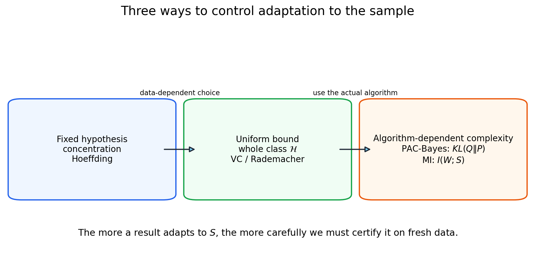
Both quantities can be more local than a worst-case count of an entire hypothesis class. But they answer different questions and provide different kinds of guarantees. PAC-Bayes usually yields a high-probability certificate for a realized sample. The basic MI bound controls the expected gap over the random sample and the algorithm's randomness.

That distinction will matter throughout the module.

12.2. From a fixed model to adaptive selection

A fixed model

Suppose $w$ is chosen before the sample $S$ is observed. Hoeffding's inequality gives

$$\Pr\left( |L(w)-\widehat L_S(w)|\ge\varepsilon \right) \le 2e^{-2n\varepsilon^2}.$$

The situation is straightforward: an average of independent bounded random variables concentrates around its expectation.

But a learned model

$$W=A(S)$$

is not fixed in advance. It was selected precisely because it looked good on $S$. We cannot insert $W$ into the fixed-$w$ bound: dependence on the sample is exactly the quantity that must be accounted for.

Uniform convergence

The classical solution is to ask for an estimate that holds simultaneously for every model in a class $\mathcal H$. For a finite class, a union bound yields

$$\Pr\left( \sup_{w\in\mathcal H} |L(w)-\widehat L_S(w)| \ge\varepsilon \right) \le 2|\mathcal H|e^{-2n\varepsilon^2}.$$

Therefore, with probability at least $1-\delta$,

$$\sup_{w\in\mathcal H} |L(w)-\widehat L_S(w)| \le \sqrt{ \frac{\ln(2|\mathcal H|/\delta)}{2n} }.$$

The price of choosing among $|\mathcal H|$ alternatives appears as $\ln|\mathcal H|$. This is already an information-theoretic hint: naming one winner among $M$ candidates takes on the order of $\log M$ bits.

For infinite classes, size is replaced by VC dimension, Rademacher complexity, norm and margin controls, and other complexity measures.

It is easy to draw an overly strong conclusion here. Uniform bounds are not "wrong for neural networks." They are correct worst-case statements for an entire class. The difficulty is that a coarse global complexity measure for a huge network often produces a numerically vacuous bound—larger than one for a risk in $[0,1]$.

A real algorithm does not explore every point in parameter space equally. SGD, architecture, pretraining, regularization, and the data itself guide it toward a much smaller region. So it is natural to ask not only

how large is the whole class?

but also

how complex is the particular output produced by this algorithm on this sample?

Adaptive selection in miniature

Return to the 32 equally good hypotheses. The hard selection rule

$$W=\arg\min_j\widehat L_S(w_j)$$

is driven almost entirely by random differences among empirical errors. In the experiment,

$$I(W;S)\approx3.24\ \text{nats},$$ $$\mathbb E[\operatorname{gen}]\approx0.087,$$

while the information bound derived in Section 12.6 is about

$$0.142.$$

Replace the hard minimum by a tempered Gibbs rule,

$$\Pr(W=j\mid S) \propto \exp\left[-\frac{\widehat L_S(w_j)}{\tau}\right].$$

As the temperature $\tau$ increases, the choice becomes less sensitive to sample-specific fluctuations. Both $I(W;S)$ and the selection bias decrease.

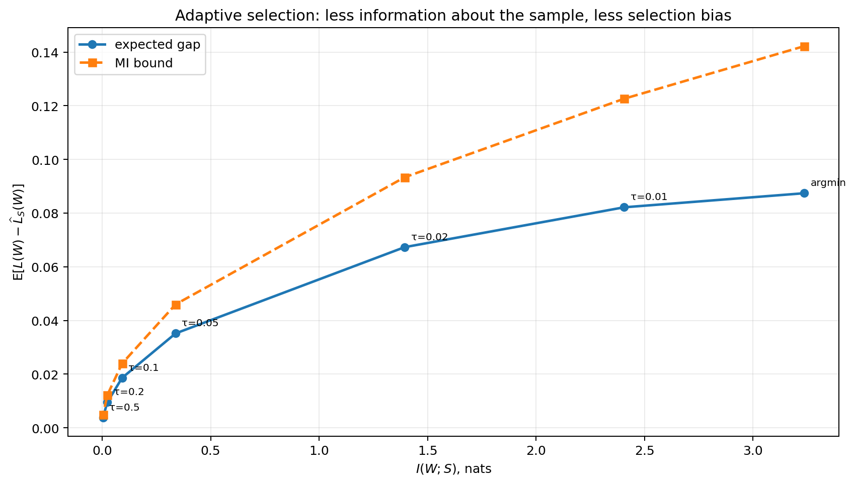
This toy example does not prove that adding noise always improves learning. It isolates a narrower mechanism: randomization can limit the amount of sample-specific information used to select the output.

12.3. PAC-Bayes: a distribution before data and a distribution after learning

PAC-Bayes changes the object being analyzed. Instead of a single learned hypothesis, it studies distributions over hypotheses or parameters.

• $P$ is a prior, fixed independently of the certifying sample $S$;
• $Q_S$ is a posterior, allowed to depend on the full sample;
• at prediction time, a model $W$ is sampled from $Q_S$.

The words prior and posterior come from Bayesian statistics, but PAC-Bayes does not require $Q_S$ to be an ordinary Bayesian posterior. They can be any probability measures satisfying the theorem's conditions.

Define the Gibbs predictor risks:

$$L(Q) = \mathbb E_{W\sim Q}[L(W)],$$ $$\widehat L_S(Q) = \mathbb E_{W\sim Q}[\widehat L_S(W)].$$

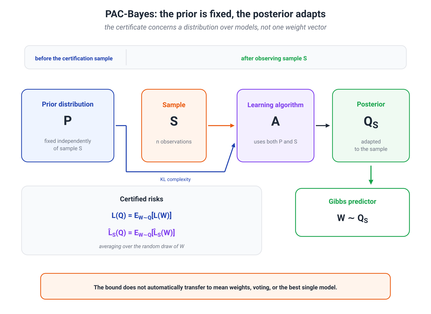
The certified object must remain explicit. The basic bound applies to a Gibbs predictor: a model is sampled from $Q$, and risk is averaged over that draw.

This is not the same as

1. a network with mean weights $\mathbb E_Q[W]$;
2. an ensemble that averages logits or probabilities;
3. a majority vote;
4. the best individual model in the support of $Q$.

Additional results can sometimes connect these predictors, but the Gibbs risk cannot be replaced by a mean-model risk merely by calling both of them an ensemble.

What the KL term pays for

The quantity

$$D_{\mathrm{KL}}(Q_S\|P)$$

measures how far the post-learning distribution moved from the reference distribution chosen before certification.

If $P$ already places substantial mass near good solutions, the posterior does not need to move far. If $Q_S$ concentrates in a region where $P$ assigns almost no mass, the cost is large.

This is not simply the distance between initial and final weights. KL depends on the full distributions, their variances, supports, and parameterization.

Why the prior cannot be trained for free on the same certifying sample

The PAC-Bayes theorem will hold simultaneously for every $Q$, so the posterior may be selected after seeing the data. The prior, however, is used in the concentration argument as a distribution independent of $S$.

If we train $P$ on the full certifying sample, choose $Q_S$ close to it, and insert the resulting small KL into the standard formula, the data have been used twice:

• once to choose the reference point;
• once to choose the posterior.

The second use is paid for by KL; the first is not.

Valid alternatives exist: sample splitting, hierarchical priors, differentially private selection, and specialized data-dependent PAC-Bayes theorems. But the dependence must appear somewhere in the guarantee.

12.4. PAC-Bayes-kl: a certificate for a realized sample

For $a,b\in[0,1]$, define the binary KL divergence

$$\operatorname{kl}(a\|b) = a\ln\frac ab +(1-a)\ln\frac{1-a}{1-b}.$$

The lowercase kl is deliberate: this is the KL divergence between Bernoulli distributions with parameters $a$ and $b$.

The theorem

Assume that

• $S\sim\mathcal D^n$ i.i.d.;
• $0\le\ell\le1$;
• $P$ is independent of $S$;
• $n\ge2$.

Then, with probability at least $1-\delta$ over $S$, simultaneously for every posterior $Q$,

$$\boxed{ \operatorname{kl} \bigl( \widehat L_S(Q)\|L(Q) \bigr) \le \frac{ D_{\mathrm{KL}}(Q\|P) + \ln\dfrac{2\sqrt n}{\delta} }{n} }.$$

This is commonly called a PAC-Bayes-kl bound; the factor $2\sqrt n$ comes from Maurer's sharpened exponential-moment estimate.

Read the formula in words.

• The left side compares observed Gibbs risk with unknown population Gibbs risk.
• The first term on the right pays for moving the posterior away from the prior.
• The second sets the confidence level.
• Division by $n$ spreads that cost over the sample size.

Let

$$c(Q,S) = \frac{ D_{\mathrm{KL}}(Q\|P) + \ln(2\sqrt n/\delta) }{n}.$$

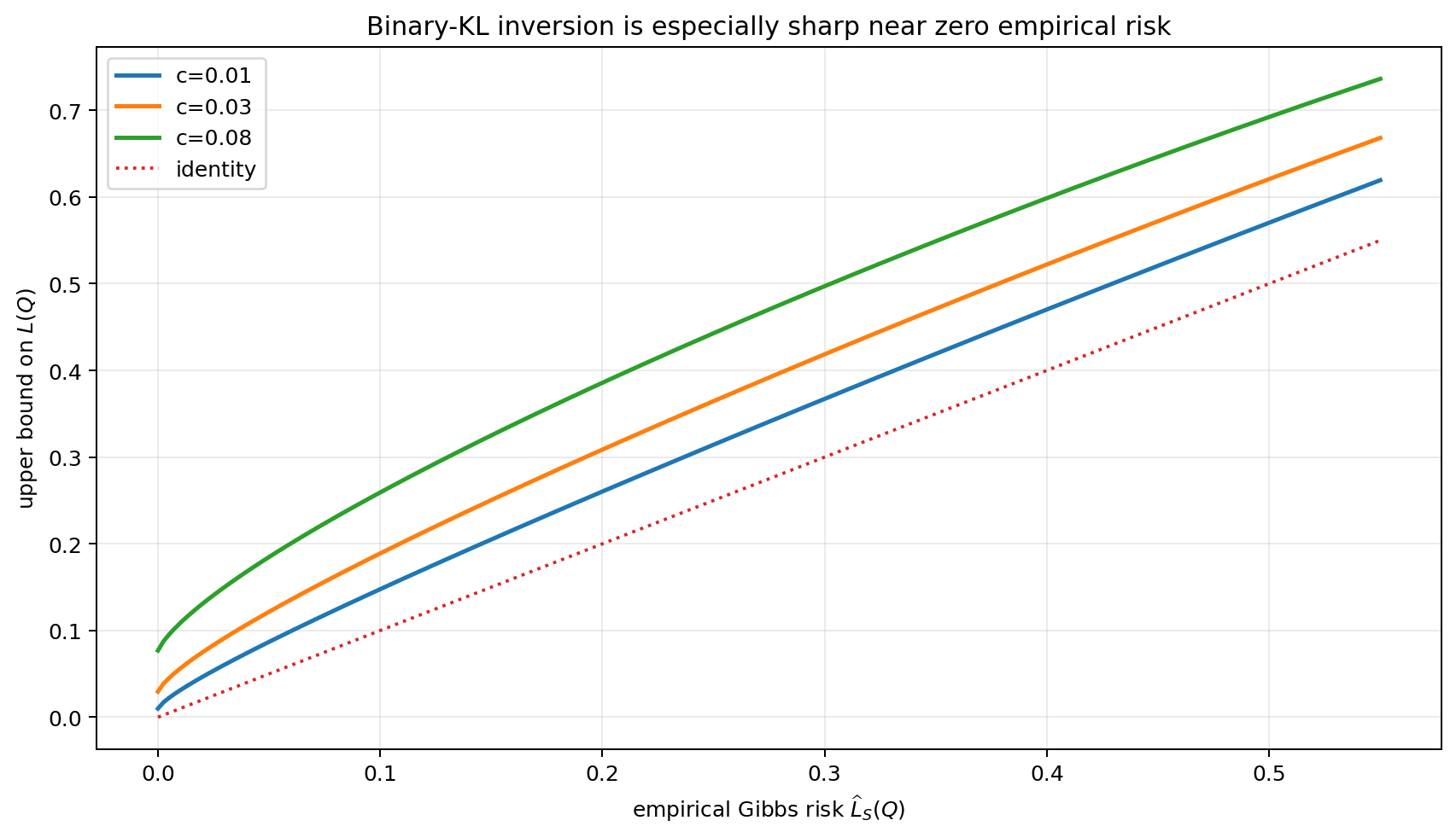
The upper certificate is obtained by numerically inverting binary KL:

$$L(Q) \le \operatorname{kl}^{-1}_{+} \bigl( \widehat L_S(Q),c(Q,S) \bigr).$$

This is not cosmetic notation. Exact inversion is particularly valuable when empirical risk is small.

Why the square-root corollary loses information

Pinsker's inequality gives

$$\operatorname{kl}(a\|b) \ge 2(a-b)^2.$$

Therefore PAC-Bayes-kl implies the simpler bound

$$L(Q) \le \widehat L_S(Q) + \sqrt{ \frac{ D_{\mathrm{KL}}(Q\|P) + \ln(2\sqrt n/\delta) }{2n} }.$$

It is easy to read, but it replaces the exact binary-KL geometry by a parabola.

If

$$\widehat L_S(Q)=0,$$

then

$$\operatorname{kl}(0\|L) =-\ln(1-L),$$

so

$$L(Q) \le 1-e^{-c} \approx c$$

for small $c$. The exact bound scales like $1/n$, while the square-root corollary only gives $1/\sqrt n$.

For example, when $c=0.01$,

$$1-e^{-c}\approx0.00995,$$

whereas Pinsker gives

$$\sqrt{c/2}\approx0.0707.$$

The difference is no longer cosmetic.

Why the theorem is true: four steps

The full proof remains in the main route because it reveals the core PAC-Bayes mechanism: moving concentration from a data-independent prior to a data-dependent posterior.

Step 1. An exponential moment for a fixed hypothesis. For each fixed $w$,

$$\mathbb E_S \exp\left[ n\operatorname{kl} \bigl( \widehat L_S(w)\|L(w) \bigr) \right] \le 2\sqrt n.$$

This is a sharpened concentration estimate for averages of bounded random variables.

Step 2. Average under the prior. Because $P$ is independent of $S$, expectations may be exchanged:

$$\mathbb E_S \mathbb E_{W\sim P} \exp\left[ n\operatorname{kl} \bigl( \widehat L_S(W)\|L(W) \bigr) \right] \le 2\sqrt n.$$

Step 3. Convert an average statement into a high-probability event. Markov's inequality implies that, with probability at least $1-\delta$,

$$\mathbb E_{W\sim P} \exp\left[ n\operatorname{kl} \bigl( \widehat L_S(W)\|L(W) \bigr) \right] \le \frac{2\sqrt n}{\delta}.$$

Step 4. Change measure. For any $Q$ and measurable $F$, the Donsker–Varadhan inequality gives

$$\mathbb E_Q[F(W)] \le D_{\mathrm{KL}}(Q\|P) + \ln\mathbb E_Pe^{F(W)}.$$

Set

$$F(w) = n\operatorname{kl} \bigl( \widehat L_S(w)\|L(w) \bigr).$$

On the event from Step 3,

$$\mathbb E_Q \operatorname{kl} \bigl( \widehat L_S(W)\|L(W) \bigr) \le \frac{ D_{\mathrm{KL}}(Q\|P) + \ln(2\sqrt n/\delta) }{n}.$$

Finally, joint convexity of binary KL yields

$$\operatorname{kl} \bigl( \widehat L_S(Q)\|L(Q) \bigr) \le \mathbb E_Q \operatorname{kl} \bigl( \widehat L_S(W)\|L(W) \bigr).$$

The theorem follows.

That is the entire mechanism: concentration for a fixed model is transferred to a post-data distribution at a KL cost.

Notice where independence of $P$ entered: Step 2. If $P=P_S$, the exchange of expectations no longer has the same form and an additional term is required.

12.5. From a certificate to a trainable distribution

PAC-Bayes can be applied after training, but its structure also suggests an objective.

For $\lambda>0$, consider

$$\mathcal F_\lambda(Q) = \widehat L_S(Q) + \frac{1}{\lambda n} D_{\mathrm{KL}}(Q\|P).$$

The Gibbs variational principle gives the exact optimizer

$$\boxed{ Q_\lambda(dw) = \frac{ P(dw)e^{-\lambda n\widehat L_S(w)} }{ \mathbb E_{W\sim P} [e^{-\lambda n\widehat L_S(W)}] } }.$$

Equivalently,

$$Q_\lambda = \arg\min_Q\mathcal F_\lambda(Q).$$

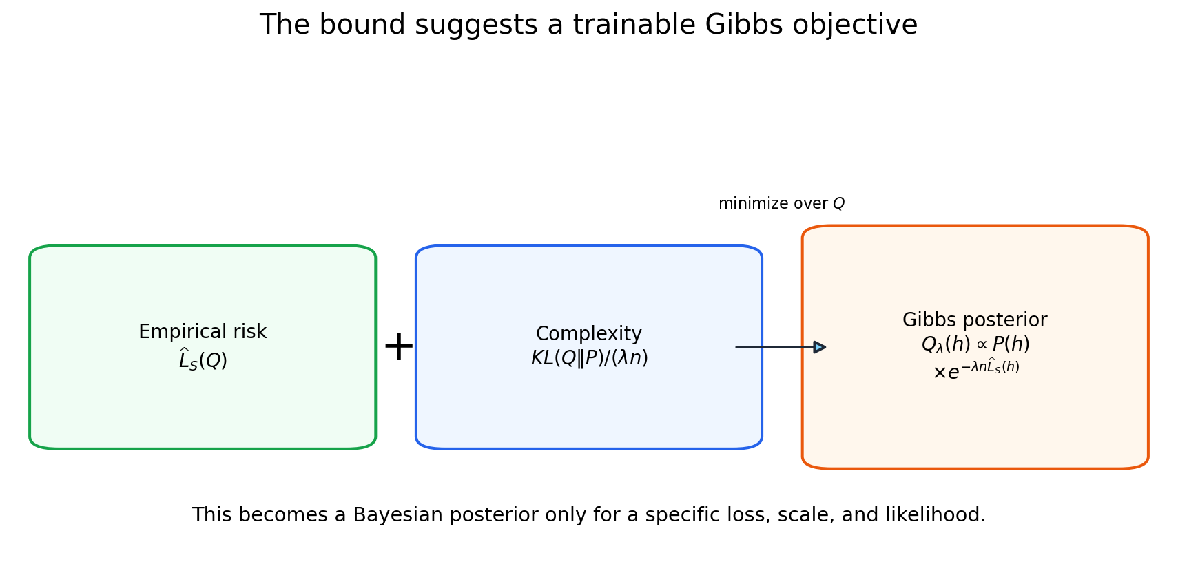
This is the same exponential tilt encountered in maximum entropy and KL-regularized policies:

• empirical risk shifts mass toward good models;
• the prior sets the reference geometry;
• KL prices a large departure;
• $\lambda$ sets the exchange rate between fit and complexity.

This is not always an ordinary Bayesian posterior

If

$$\lambda n\widehat L_S(w) = -\log p(S\mid w)$$

up to a $w$-independent constant, then $Q_\lambda$ coincides with the Bayesian posterior.

For an arbitrary loss, it is a generalized Gibbs posterior, not an ordinary likelihood update.

Moreover, $Q_\lambda$ exactly minimizes $\mathcal F_\lambda$, but it is not automatically the exact minimizer of every PAC-Bayes bound one might choose. Practical methods may minimize a differentiable certificate, its numerical inversion, or a convenient surrogate. The common motif is empirical risk plus an information price.

Gaussian distributions over weights

Let

$$P = \mathcal N \bigl( \mu_P, \operatorname{diag}(\sigma_P^2) \bigr),$$ $$Q = \mathcal N \bigl( \mu_Q, \operatorname{diag}(\sigma_Q^2) \bigr).$$

Then

$$\begin{aligned} D_{\mathrm{KL}}(Q\|P) = \frac12\sum_j \Bigg[ &\frac{\sigma_{Q,j}^2}{\sigma_{P,j}^2} + \frac{(\mu_{Q,j}-\mu_{P,j})^2}{\sigma_{P,j}^2} -1\\ &+ \ln\frac{\sigma_{P,j}^2}{\sigma_{Q,j}^2} \Bigg]. \end{aligned}$$

The quadratic term in the means does resemble $L_2$ regularization. But it is only one component of KL. A full PAC-Bayes setup also controls variances and certifies a distribution of predictors.

The accurate statement is therefore:

A Gaussian PAC-Bayes complexity term contains an $L_2$-like component, but ordinary deterministic weight decay is not the same as full PAC-Bayes training.

The same caution applies to dropout. It introduces randomness, but a particular PAC-Bayes guarantee still requires explicit choices of $P$, $Q$, risk, and certification procedure.

Why a point model often has infinite KL

If $P$ has a continuous density and

$$Q=\delta_{w_*},$$

then

$$D_{\mathrm{KL}}(\delta_{w_*}\|P)=\infty.$$

The point mass is not absolutely continuous with respect to the continuous prior.

Practical certificates therefore usually use

• a stochastic distribution around the weights;
• discretization or quantization;
• a prior with an appropriate atomic component;
• separate results for majority votes or deterministic predictors.

Randomization is not a magical source of generalization. It makes the certified object well defined and creates a trade-off between predictive robustness and KL cost.

12.6. MI bounds: learning as a channel from sample to model

Now remove the manually chosen prior and view the entire learning algorithm as a channel

$$S\longrightarrow W.$$

The algorithm may be random because of initialization, minibatch order, dropout, injected noise, or an explicit draw from a posterior distribution.

The mutual information

$$I(W;S) = D_{\mathrm{KL}} \left( P_{W,S} \|P_W\otimes P_S \right)$$

measures how much the output distribution changes when the particular training sample is known.

This is close to the informal idea of "how much the model memorized," but a more precise reading is

$I(W;S)$ measures statistical dependence between the algorithm's output and the full training sample.

It does not directly tell us which examples are reconstructable, whether privacy has been violated, or whether semantically important facts were retained. Those require separate operational criteria.

The Xu–Raginsky theorem

Assume that, for every fixed $w$, the centered loss

$$\ell(w,Z)-L(w)$$

is $\sigma$-sub-Gaussian:

$$\ln \mathbb E_Z \exp\left[ \lambda(\ell(w,Z)-L(w)) \right] \le \frac{\lambda^2\sigma^2}{2}$$

for every $\lambda\in\mathbb R$.

Then

$$\boxed{ \left| \mathbb E \left[ L(W)-\widehat L_S(W) \right] \right| \le \sqrt{ \frac{2\sigma^2 I(W;S)}{n} } }.$$

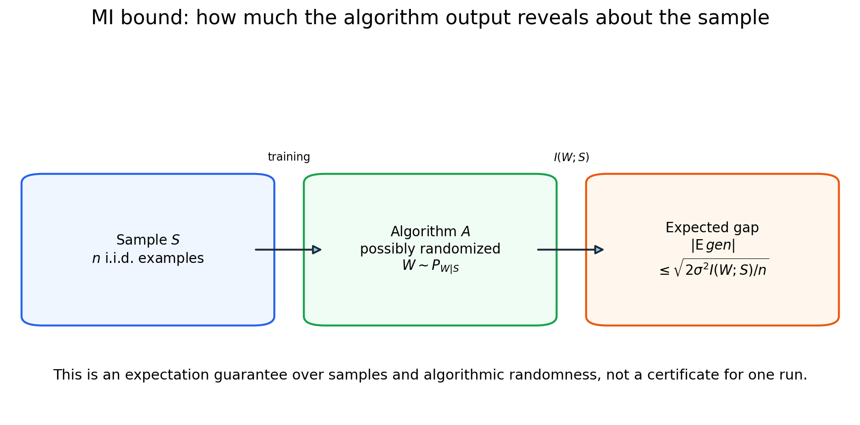
If $0\le\ell\le1$, Hoeffding's lemma permits

$$\sigma^2=\frac14,$$

which gives

$$\left| \mathbb E\operatorname{gen} \right| \le \sqrt{ \frac{I(W;S)}{2n} }.$$

Where the formula comes from

Under the product distribution $P_S\otimes P_W$, the model $W$ is independent of the sample. For fixed $W$, empirical risk concentrates around population risk with sub-Gaussian parameter $\sigma/\sqrt n$.

Actual learning uses the joint distribution $P_{S,W}$. The change-of-measure inequality from Module 11 compares expectations under the joint distribution and under the product of marginals. Its cost is

$$D_{\mathrm{KL}} \left( P_{S,W} \|P_S\otimes P_W \right) = I(W;S).$$

Optimizing the exponential-moment parameter produces the square root. As in PAC-Bayes, concentration is transferred from an independent setting to a dependent one. Here the cost is not KL to a chosen prior but the mutual information of the algorithm itself.

A numerical adaptive-selection example

For hard selection among 32 equally good hypotheses, the experiment gives

$$I(W;S)\approx3.235\ \text{nats},$$

and, for $n=80$,

$$\sqrt{\frac{I(W;S)}{2n}} \approx0.142,$$

while the observed expected gap is about $0.087$.

The bound is not exact, but it tracks the correct mechanism: as the Gibbs-selection temperature increases, dependence on sample-specific fluctuations decreases, and the selection bias decreases with it.

What type of guarantee did we obtain?

The basic MI result controls

$$\mathbb E_{S,W} \left[ L(W)-\widehat L_S(W) \right].$$

It is an expectation bound. It is not automatically a high-probability certificate for one trained model and one realized sample.

It also concerns the selected loss. A small expected gap in cross-entropy does not guarantee a small gap in factual correctness, safety, or human preference.

Why a deterministic real-valued model can have infinite MI

If $W$ takes finitely many values and is a deterministic function of $S$, then

$$I(W;S)=H(W)<\infty.$$

But if $W$ is an exact real-valued vector deterministically computed from a continuous sample, the joint law of $(S,W)$ is often singular with respect to $P_S\otimes P_W$. Then

$$I(W;S)=\infty.$$

The algorithm may generalize well while the basic bound remains vacuous. That is a limitation of the chosen information measure, not a proof of poor generalization.

Adding noise may make MI finite, but it changes the algorithm and its risk. Noise cannot be inserted only into the proof while the original deterministic predictor is certified without an additional argument.

Individual-sample MI

A more local estimate uses the dependencies $I(W;Z_i)$:

$$\left| \mathbb E\operatorname{gen} \right| \le \frac1n \sum_{i=1}^n \sqrt{ 2\sigma^2 I(W;Z_i) }.$$

It can be substantially tighter than the global bound: each example may influence the output only weakly even when total dependence $I(W;S)$ is large or infinite.

12.7. The exact decomposition connecting PAC-Bayes and MI

Let the learning algorithm define the conditional distribution

$$Q_S=P_{W\mid S},$$

and let $P_W$ be the marginal distribution of its output over random training samples.

For any fixed prior $P$ for which the relevant divergences are finite,

$$\boxed{ \mathbb E_S D_{\mathrm{KL}}(Q_S\|P) = I(W;S) + D_{\mathrm{KL}}(P_W\|P) }.$$

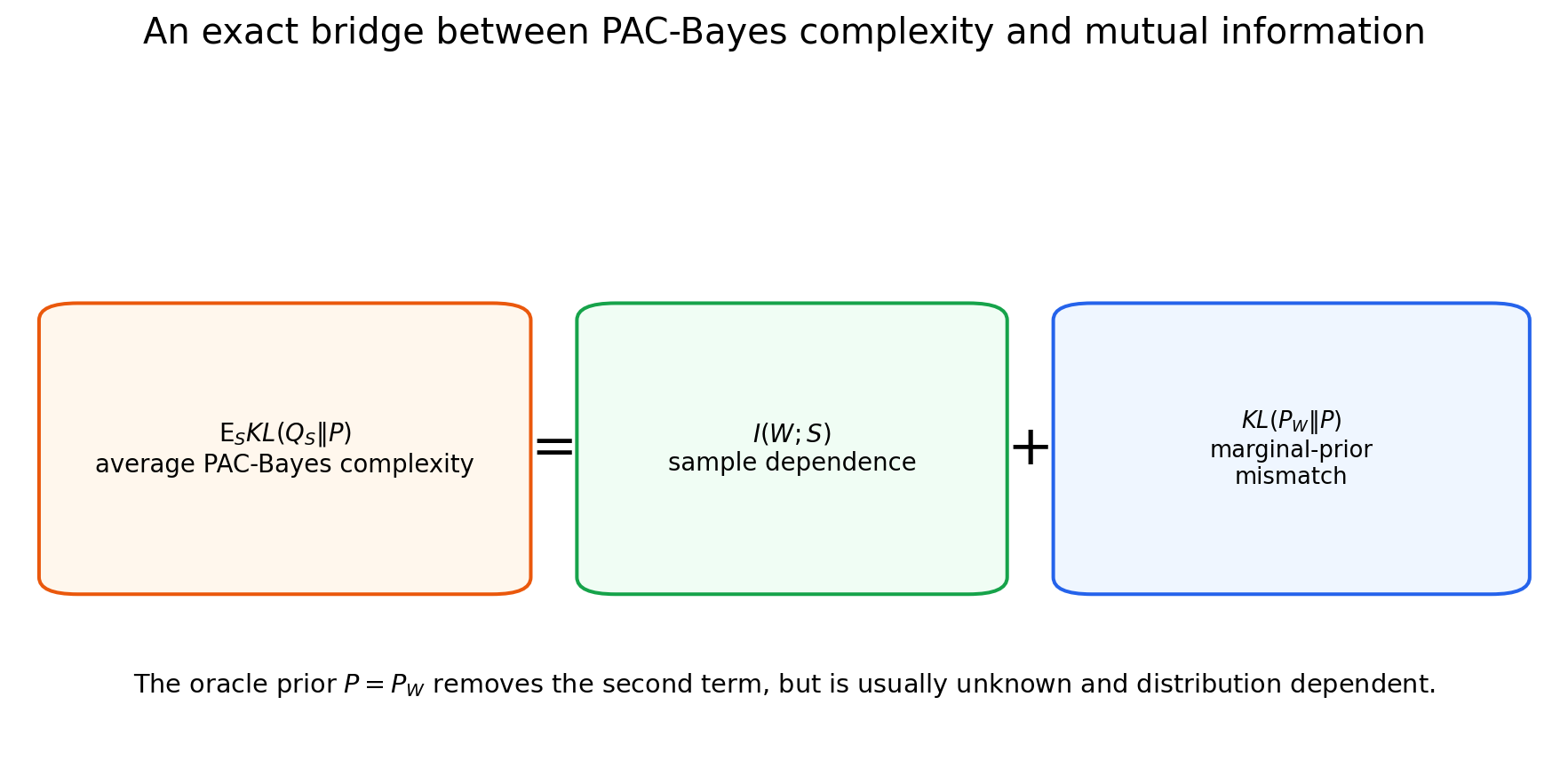
This is exact bookkeeping, not an analogy.

• $I(W;S)$ is the unavoidable average price of dependence on the sample;
• $D_{\mathrm{KL}}(P_W\|P)$ is the extra price of choosing a reference distribution that mismatches the algorithm's typical output distribution.

Proof

Add and subtract the log density of $P_W$:

$$\begin{aligned} \mathbb E_{S,W} \ln\frac{dQ_S}{dP}(W) &= \mathbb E_{S,W} \ln\frac{dQ_S}{dP_W}(W) + \mathbb E_{S,W} \ln\frac{dP_W}{dP}(W)\\ &= I(W;S) + D_{\mathrm{KL}}(P_W\|P). \end{aligned}$$

The oracle prior

The quantity

$$\mathbb E_S D_{\mathrm{KL}}(Q_S\|P)$$

is minimized by

$$P=P_W.$$

The mismatch term then vanishes and average PAC-Bayes complexity equals mutual information.

Why not simply use $P_W$? In principle, if the data distribution $\mathcal D$ and the algorithm are fully known, $P_W$ is fixed before the current sample and is a valid reference. The practical problem is that it depends on the unknown distribution of all possible training samples and is generally unavailable.

If $P_W$ is estimated from the same certifying sample, the prior becomes data-dependent and the standard theorem requires a correction.

What is unified and what remains different

The identity explains why PAC-Bayes and MI often suggest similar regularizers. Their guarantees still differ.

Thus "MI is averaged PAC-Bayes" is a useful first map, but not a substitute for either theorem.

12.8. Connections to MDL, Information Bottleneck, and KL-regularized policies

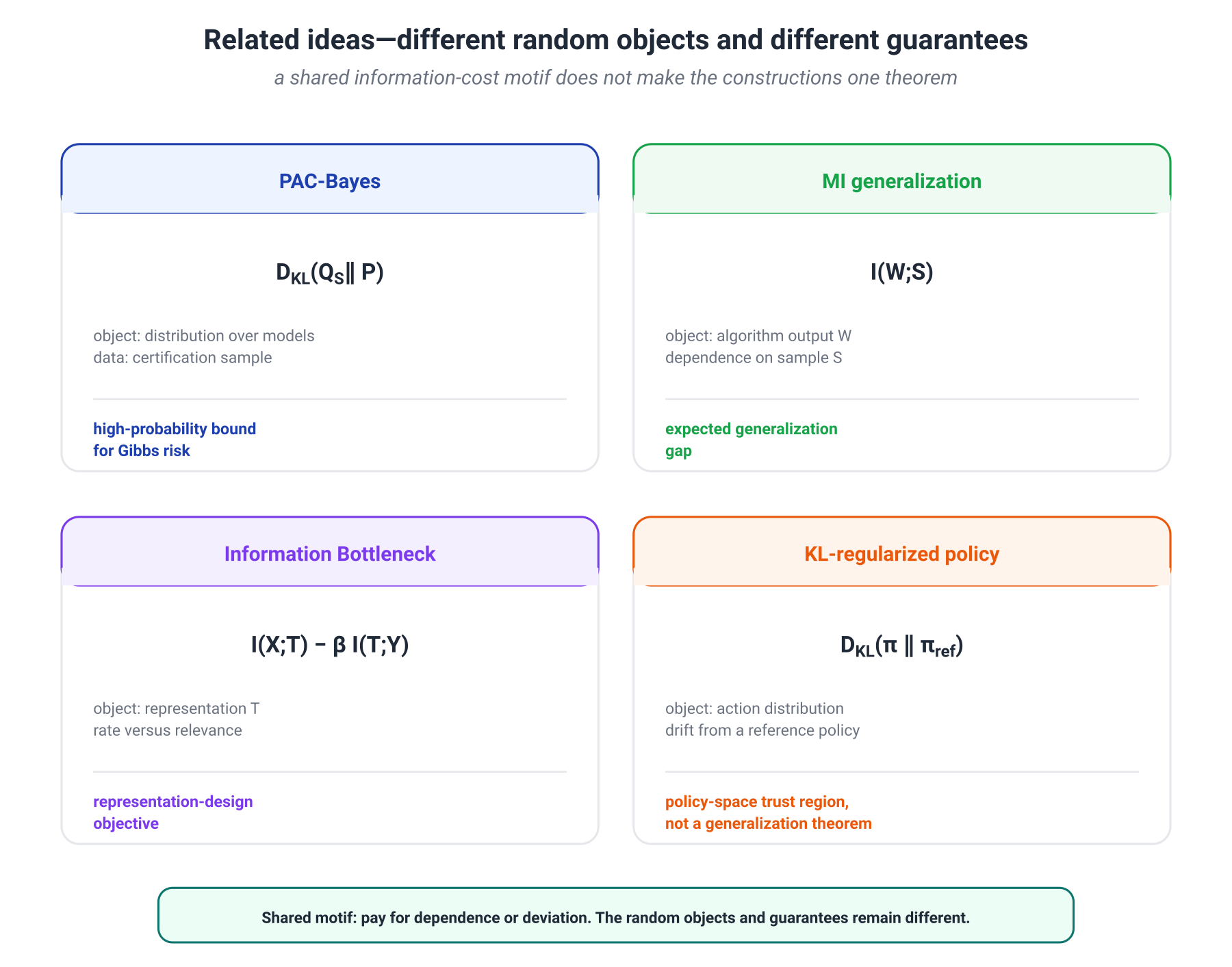
The information-theoretic constructions from earlier modules are genuinely related. The safest way to see the relationship is to write down the random variables and the operational meaning of each KL.

PAC-Bayes and MDL

Suppose the class is discrete and

$$Q=\delta_w, \qquad P(w)>0.$$

Then

$$D_{\mathrm{KL}}(\delta_w\|P) =-\ln P(w).$$

In bits,

$$-\log_2P(w),$$

which is the ideal code length of the hypothesis under the prior code.

This is an exact bridge: PAC-Bayes pays for describing the selected model relative to a declared code.

But MDL is broader than one formula. It includes two-part, mixture, and prequential codes; continuous parameters require a precision convention or a stochastic code; and the data code can be organized in several ways.

MI generalization bounds and Information Bottleneck

Information Bottleneck studies

$$I(X;T),$$

where $X$ is an individual input and $T$ its representation.

Generalization theory studies

$$I(W;S),$$

where $S$ is the entire training sample and $W$ the algorithm's output.

Both quantities penalize dependence on details of an input object, but the objects and tasks differ:

• IB asks how much information a representation retains about an input;
• the MI bound asks how strongly a learned output depends on the realized training sample.

Small $I(X;T)$ is not by itself a proof of small $I(W;S)$ and does not automatically yield a generalization bound. The old slogan that MI bounds "strictly prove IB" was too strong. A better statement is that both theories use an information-limitation principle; a direct implication requires an additional model of learning.

PAC-Bayes KL and the KL anchor in RLHF

In PAC-Bayes,

$$D_{\mathrm{KL}} (Q_{\text{models}}\|P_{\text{models}})$$

compares distributions over models or weights.

In KL-regularized RLHF,

$$D_{\mathrm{KL}} \bigl( \pi(\cdot\mid x) \|\pi_{\mathrm{ref}}(\cdot\mid x) \bigr)$$

compares output distributions of policies at a fixed context.

The algebra looks similar because both problems use an exponential tilt relative to a reference measure. The random objects are not the same.

A second boundary matters after Module 8: PAC-Bayes controls the move from empirical to population risk for a specified loss. If a proxy reward is systematically misaligned with the true objective, a small generalization gap for the proxy does not repair that bias.

12.9. Building a practical PAC-Bayes certificate

The theorem becomes an engineering tool only when every random object is defined without ambiguity.

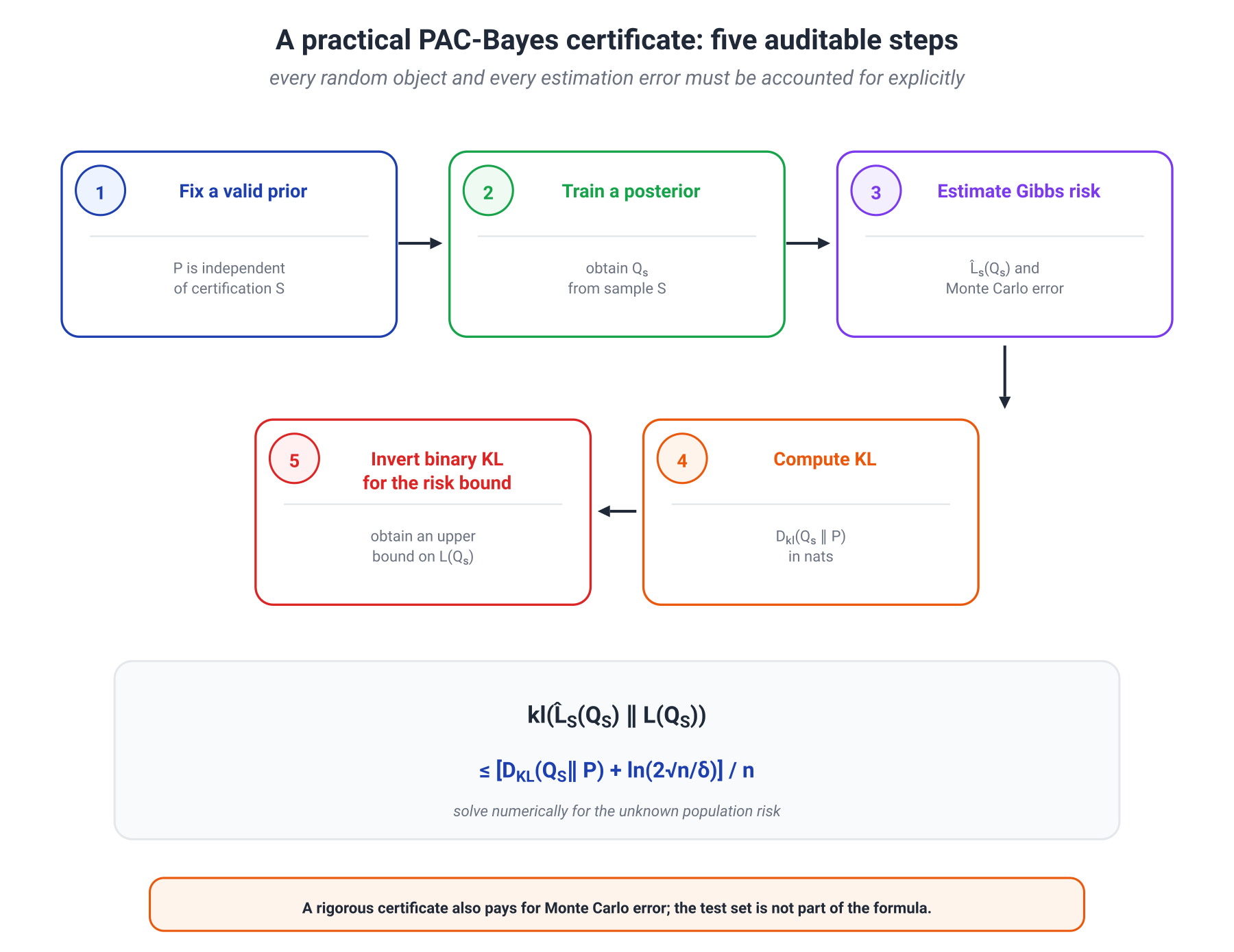
Step 1. Fix the certified predictor and loss

Decide what will actually be deployed:

• a Gibbs predictor;
• a posterior ensemble;
• a majority vote;
• a deterministic network.

The basic bound applies to Gibbs risk. Another predictor requires a separate connection.

The loss must also be bounded and explicit. One cannot train with cross-entropy, evaluate 0–1 error, and silently substitute one for the other in a theorem.

Step 2. Fix a valid prior

The simplest choice is a prior selected before the certifying data.

A stronger practical option is sample splitting:

1. use $S_0$ to build an informative prior;
2. use an independent subset $S_1$ to train $Q$ and certify conditionally on $S_0$.

The trade-off is immediate: the prior improves, but the effective certification sample becomes smaller.

Step 3. Train a distribution rather than only a point

For a diagonal Gaussian $Q$, both means and variances are optimized. Variances that are too small preserve fit but incur a large KL. Variances that are too large reduce some complexity terms but damage predictions.

The certificate therefore searches not merely for a "flat minimum" but for a concrete compromise between robustness of the stochastic predictor and cost relative to $P$.

Step 4. Certify empirical Gibbs risk

The expectation over $Q$ is often estimated by Monte Carlo. A finite number of posterior samples introduces another statistical error.

Averaging ten sampled networks and inserting that number directly into the theorem is not a rigorous certificate. One needs a separate confidence bound for empirical Gibbs risk or an analytic expectation.

Step 5. Compute KL and invert binary KL

For diagonal Gaussians, $D_{\mathrm{KL}}(Q\|P)$ is analytic. The PAC-Bayes-kl relation is then inverted numerically.

In the module's stochastic linear-classifier experiment,

$$\widehat L_S(Q)\approx0.227,$$ $$D_{\mathrm{KL}}(Q\|P)\approx12.67\ \text{nats},$$

and, at $\delta=0.05$,

$$L(Q)\le0.272.$$

The diagnostic test Gibbs risk is approximately

$$0.225.$$

The test set is not part of the certificate; it is used only to diagnose the experiment.

What has been achieved for deep networks

Dziugaite and Roy showed that direct optimization of a PAC-Bayes bound can produce nonvacuous certificates for stochastic deep networks with millions of parameters. A later PAC-Bayes with Backprop method reported, under its MNIST protocol, test error around $1.4\%$ together with a certificate around $2.3\%$.

This is an important counterexample to the claim that every theoretical bound for a deep network must exceed one. It is not a universal explanation of deep learning:

• the result depends on architecture, parameterization, and prior;
• the certified object is stochastic;
• tightness on MNIST does not transfer automatically to LLMs;
• a computable certificate can still be much looser than held-out evaluation.

The right conclusion is both narrower and stronger: PAC-Bayes can provide a real numerical guarantee for a large model when the training and certification pipeline is deliberately designed for that purpose.

12.10. Mathematical deepening: more local information costs

This section is not required for the main route. It shows how the theory addresses two weaknesses of the basic formulas: a prior is hard to choose before data, and $I(W;S)$ may be infinite for deterministic continuous models.

Data-dependent priors

Several strategies are valid.

Sample splitting. Build $P$ from $S_0$ and apply the theorem conditionally to an independent subset $S_1$.

Hierarchical priors. Selecting one member of a family of priors is encoded at a higher level and paid for by an additional KL or union-bound term.

Differentially private selection. If the mechanism constructing $P_S$ has controlled dependence on the data, that dependence can be incorporated into a PAC-Bayes guarantee.

Specialized data-dependent PAC-Bayes theorems. These explicitly add a term measuring how the reference distribution used the data.

The common rule remains

Data used to reduce the complexity term cannot disappear from the accounting for free.

Individual-sample MI

The global quantity $I(W;S)$ may hide local structure. The chain rule gives

$$I(W;S) = \sum_{i=1}^n I(W;Z_i\mid Z_{<i}),$$

but a bound involving

$$\sqrt{I(W;S)}$$

first adds all contributions and then takes one square root.

An individual-sample bound instead uses

$$\frac1n \sum_{i=1}^n \sqrt{I(W;Z_i)}.$$

When every example has only a weak effect, this local aggregation can be substantially smaller.

Conditional mutual information

Construct a supersample

$$\widetilde S = \bigl( \widetilde Z_{i,0}, \widetilde Z_{i,1} \bigr)_{i=1}^n$$

with two independent candidates for each position. Let

$$U=(U_1,\ldots,U_n), \qquad U_i\sim\operatorname{Bernoulli}(1/2),$$

and build the actual training sample as

$$S_U = \bigl( \widetilde Z_{i,U_i} \bigr)_{i=1}^n.$$

The algorithm returns

$$W=A(S_U).$$

Conditional information complexity measures

$$I(W;U\mid\widetilde S).$$

Its operational meaning is clear: if both candidate samples at every position are known, how much does the learned output reveal about the bits $U_i$ that identify which examples were actually used for training?

For a deterministic algorithm this quantity is still finite:

$$I(W;U\mid\widetilde S) \le H(U) = n\ln2.$$

That is why CMI can remain meaningful when ordinary $I(W;S)$ is infinite for exact real-valued weights.

CMI connects the information-theoretic view to VC dimension, compression schemes, and differential privacy. It is not automatically an easy metric to compute for a large neural network. It is a sharper theoretical object, not a ready-made dashboard number.

12.12. What to take away

The training sample serves two roles: it is used to choose a model and to estimate that model's performance. This reuse makes the winner's estimate optimistic.

PAC-Bayes pays for adaptivity relative to a declared reference distribution:

$$\operatorname{kl} \bigl( \widehat L_S(Q)\|L(Q) \bigr) \lesssim \frac{ D_{\mathrm{KL}}(Q\|P) + \ln(1/\delta) }{n}.$$

The MI bound pays for average dependence of the algorithm's output on the sample:

$$|\mathbb E\operatorname{gen}| \lesssim \sqrt{ \frac{I(W;S)}{n} }.$$

They are connected by the exact identity

$$\mathbb E_S D_{\mathrm{KL}}(Q_S\|P) = I(W;S) + D_{\mathrm{KL}}(P_W\|P).$$

But the complete map matters more than a single slogan.

• PAC-Bayes usually gives a high-probability certificate for a Gibbs predictor.
• The basic MI bound usually controls an algorithm's expected gap.
• A prior trained on the certifying data requires a separate information charge.
• $I(W;S)$ is not the $I(X;T)$ of Information Bottleneck.
• KL over weights is not KL between RLHF policies.
• A small proxy-loss generalization gap does not remove bias in the proxy itself.
• A nonvacuous bound proves something nontrivial but need not be tight enough for model selection.

This is not a list of defensive caveats. It is a working discipline. Information-theoretic generalization becomes useful when we name precisely

1. the random sample;
2. the algorithm's output;
3. the certified predictor;
4. the loss;
5. the type of probabilistic guarantee;
6. the adaptivity cost that can actually be computed.

That discipline will matter even more in Module 13. There, the words channel, compression, search, and information will be applied to LLM reasoning, and each bridge must be distinguished from a direct theorem.

Main references

1. D. McAllester, Some PAC-Bayesian Theorems, COLT 1998; PAC-Bayesian Stochastic Model Selection, 2003.
2. A. Maurer, A Note on the PAC Bayesian Theorem, 2004.
3. O. Catoni, PAC-Bayesian Supervised Classification, 2007.
4. D. Russo and J. Zou, Controlling Bias in Adaptive Data Analysis Using Information Theory, 2016.
5. A. Xu and M. Raginsky, Information-Theoretic Analysis of Generalization Capability of Learning Algorithms, 2017.
6. G. K. Dziugaite and D. M. Roy, Computing Nonvacuous Generalization Bounds for Deep (Stochastic) Neural Networks, 2017.
7. G. K. Dziugaite and D. M. Roy, Data-Dependent PAC-Bayes Priors via Differential Privacy, 2018.
8. O. Rivasplata, V. M. Tankasali, and C. Szepesvári, PAC-Bayes with Backprop, 2019.
9. Y. Bu, S. Zou, and V. V. Veeravalli, Tightening Mutual Information Based Bounds on Generalization Error, 2019.
10. T. Steinke and L. Zakynthinou, Reasoning About Generalization via Conditional Mutual Information, 2020.