Module 11. Comparing distributions: f-divergences, variational critics, and Wasserstein distance

How to read this module. The main route is Sections 11.1–11.9. We first build the family of f-divergences, then show how classifiers and variational critics recover density ratios from samples. The same mechanism leads to GANs, f-GAN, MINE, and InfoNCE. Section 11.8 changes the lens and adds geometry through IPMs, Wasserstein distance, and MMD. Section 11.10 is an optional mathematical deepening on singular measure components, joint convexity, and the exact conditions behind the dual representation.

11.1. From two sample sets to a distribution-comparison problem

KL has been the workhorse of the preceding modules. It appeared in cross-entropy, mutual information, the ELBO, the Information Bottleneck, KL-regularized policies, and MDL. Modern ML often presents a more awkward situation, however: we can sample from two distributions but cannot evaluate their densities.

This is the usual setting for an implicit generator. It can quickly produce

$$X=G_\theta(Z),$$

while the pointwise value $q_\theta(x)$ is typically unavailable. The expression

$$D_{\mathrm{KL}}(P\|Q_\theta) = \mathbb E_P\log\frac{p(X)}{q_\theta(X)}$$

is still mathematically meaningful, but it does not directly become a computable loss.

Consider a much smaller example. A first source emits $a$ and $b$ with probabilities

$$P=(0.8,0.2),$$

and a second source emits them with probabilities

$$Q=(0.2,0.8).$$

If the two sources are equally likely a priori, the optimal source classifier returns

$$\Pr(P\mid a)=0.8, \qquad \Pr(P\mid b)=0.2.$$

Its logits are $\log4$ and $-\log4$. This already hints at the central mechanism: an ideal classifier does more than distinguish two sample sets; it encodes their probability ratio. We derive the exact statement in Section 11.4.

The same pattern occurs in many ML problems:

• the data distribution $P_{\mathrm{data}}$ is compared with a generator distribution $Q_\theta$;
• the joint distribution $P_{XY}$ is compared with the product $P_X\otimes P_Y$ when estimating mutual information;
• representation distributions are compared before and after distribution shift;
• two sample sets are compared in a two-sample test;
• a reference policy is compared with an updated policy.

These settings raise three separate questions.

1. What should count as distributional error? Missing mass, extra mass, and geometric displacement are not the same failure.
2. How can the discrepancy be estimated from samples? This is where classifiers and variational critics enter.
3. Does the sample space itself carry useful geometry? f-divergences use probability ratios, whereas Wasserstein distance also uses distances between points.

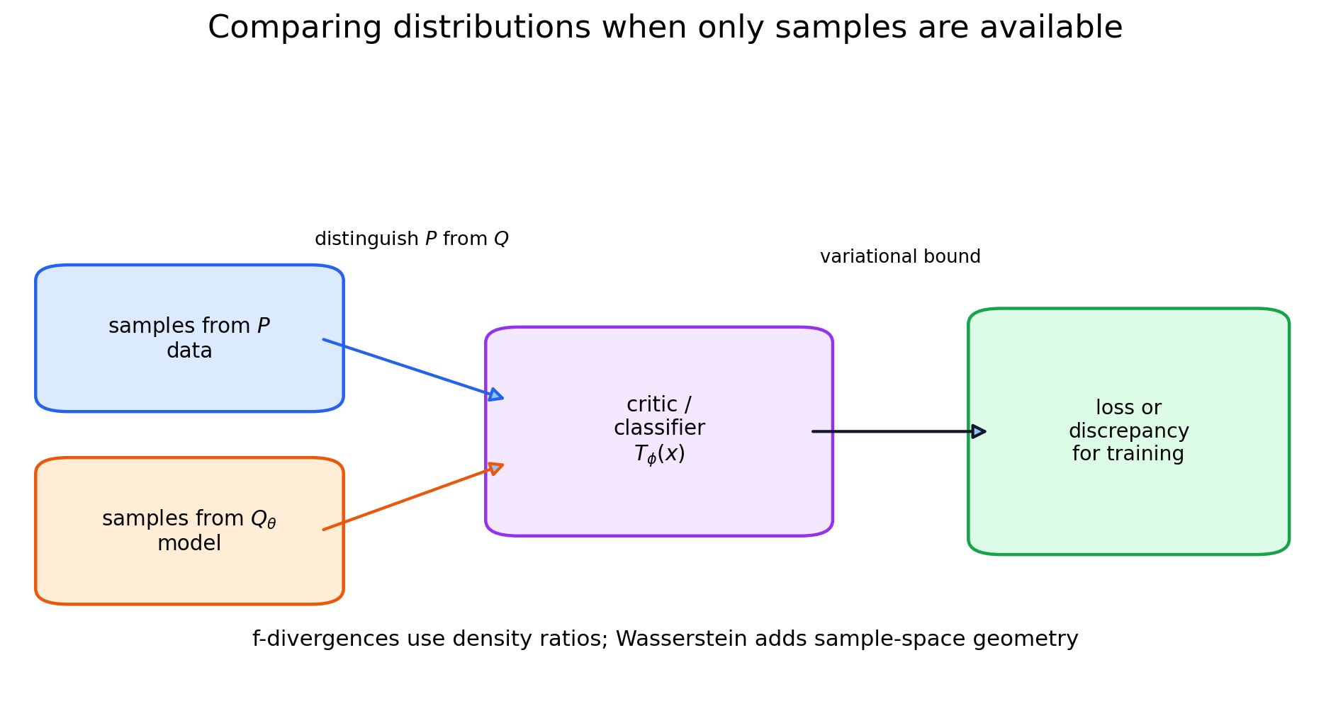
The main construction of the module is:

A variational critic turns an inaccessible density ratio into a trainable sample-based problem.

It helps to see the whole ladder before studying its steps:

$$\text{population discrepancy} \;\longrightarrow\; \text{best critic in a chosen class} \;\longrightarrow\; \text{critic fitted on finite data}.$$

The first arrow may leave a variational gap if the function class is too small. The second adds statistical and optimization error. This does not make critics useless; it tells us exactly what quantity a training run has produced.

Unless stated otherwise, logarithms are natural and logarithmic quantities are measured in nats.

11.2. f-divergences: one template, different penalties

Let $P$ and $Q$ have densities $p$ and $q$ with respect to a common base measure. Along the main route, assume for now that $P\ll Q$. Define the density ratio

$$r(x)=\frac{p(x)}{q(x)}.$$

It has a direct interpretation:

• $r(x)=1$: the two distributions assign the same relative mass at $x$;
• $r(x)>1$: $Q$ under-allocates mass relative to $P$;
• $r(x)<1$: $Q$ allocates more mass than $P$.

Choose a convex function

$$f:(0,\infty)\to\mathbb R, \qquad f(1)=0.$$

It specifies how costly each density-ratio value should be. The corresponding f-divergence is

$$\boxed{ D_f(P\|Q) = \int q(x) f\!\left(\frac{p(x)}{q(x)}\right)dx = \mathbb E_Q[f(r(X))] }.$$

In this sense, $f$ is a penalty schedule for density-ratio errors. Different schedules yield different discrepancies.

Why the divergence is nonnegative

Because

$$\mathbb E_Q[r] = \int q\frac pq = 1,$$

Jensen's inequality gives

$$D_f(P\|Q) = \mathbb E_Q[f(r)] \ge f(\mathbb E_Qr) =f(1)=0.$$

There is a useful subtlety here. The generator $f(t)$ itself need not be nonnegative at every $t$. What is nonnegative is its average score under the constraint $\mathbb E_Qr=1$. This is why equivalent generators may dip below zero without producing a negative divergence.

Equality always holds when $P=Q$. For the converse implication, $f$ must be sufficiently strictly convex on the realized range of $r$.

Main examples

We use the following normalization throughout the course:

With this normalization,

$$0\le H^2(P,Q)\le1, \qquad 0\le\operatorname{TV}(P,Q)\le1, \qquad 0\le D_{\mathrm{JS}}(P,Q)\le\log2.$$

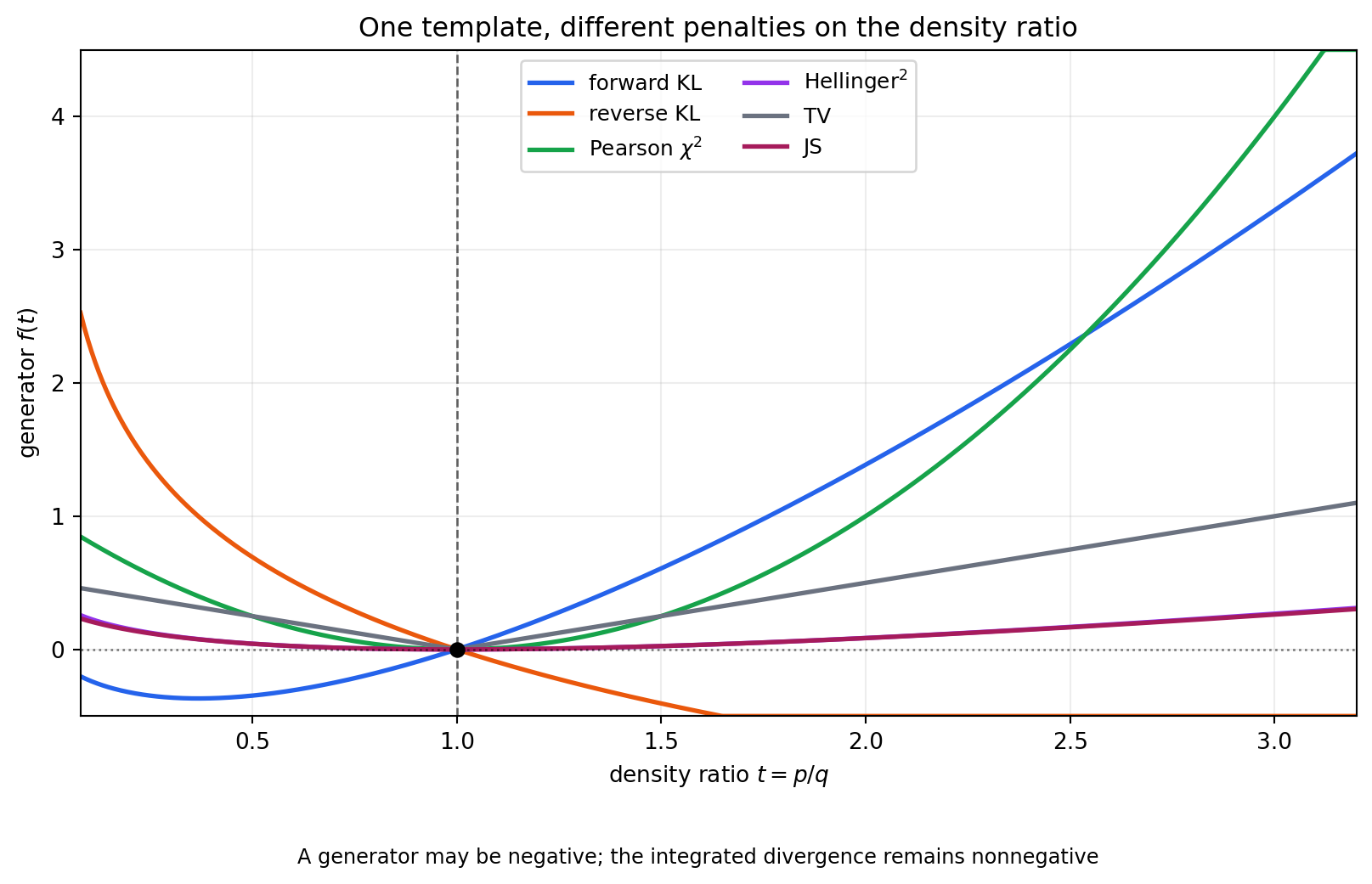
Why the generator is not unique

Replacing $f$ by

$$\widetilde f(t)=f(t)+a(t-1)$$

does not change the divergence, because

$$\mathbb E_Q[a(r-1)] =a(\mathbb E_Qr-1)=0.$$

Hence

$$D_{\widetilde f}(P\|Q)=D_f(P\|Q).$$

This is why tables sometimes display different-looking formulas for the same discrepancy: the formulas differ by a linear term that vanishes after averaging.

A neighboring family: power and Rényi divergences

For $\alpha\ne0,1$, the convex generator

$$f_\alpha(t) = \frac{t^\alpha-\alpha t+\alpha-1} {\alpha(\alpha-1)}$$

defines a family of power f-divergences. The limits $\alpha\to1$ and $\alpha\to0$ give generators that are affine-equivalent to forward and reverse KL.

For $\alpha>0$, $\alpha\ne1$, Rényi divergence,

$$D_\alpha^{\mathrm R}(P\|Q) = \frac1{\alpha-1} \log\int p^\alpha q^{1-\alpha},$$

is a monotone transformation of the corresponding power f-divergence and therefore induces the same ordering of distribution pairs for fixed $\alpha$, but it does not generally have the form $\mathbb E_Q[f(p/q)]$. Properties of all f-divergences cannot be transferred to Rényi divergence merely because the notation looks similar.

11.3. What f-divergences can see

An f-divergence tracks how one probability measure reweights another. The construction explains both its strength and its natural boundary.

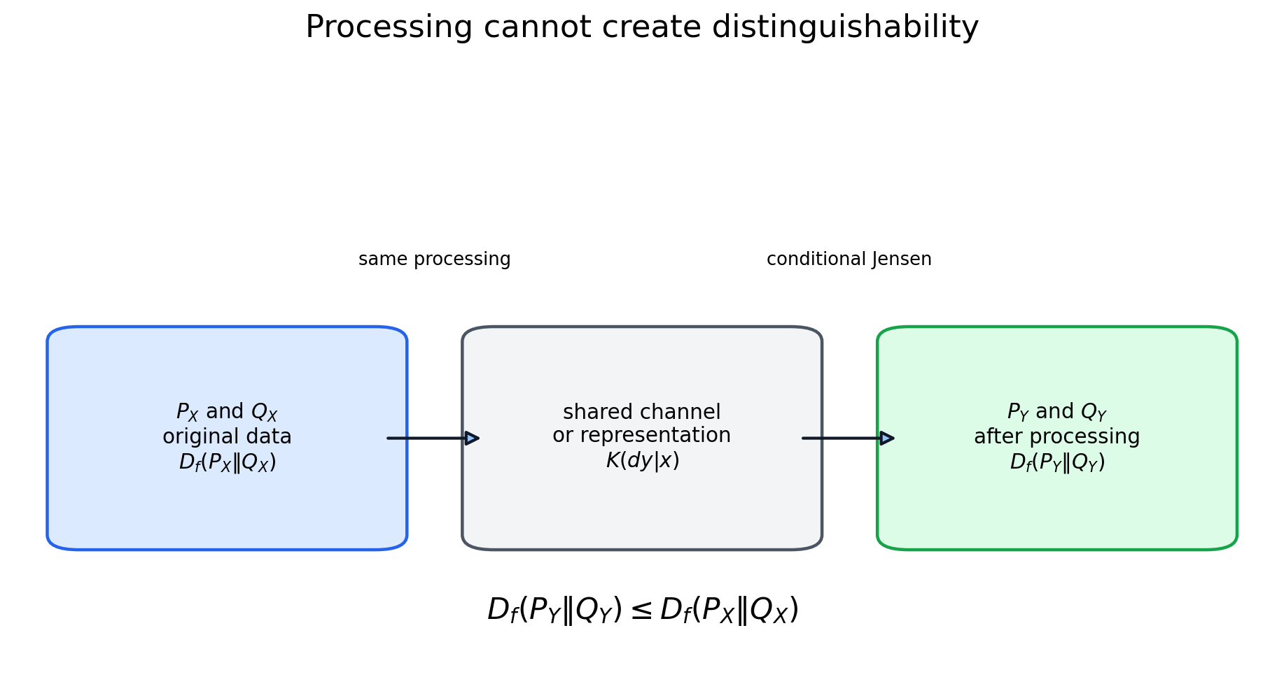
Processing cannot increase distinguishability

Apply the same stochastic channel $K(dy\mid x)$ to $P$ and $Q$, and denote the output distributions by $P_Y$ and $Q_Y$. Then

$$\boxed{ D_f(P_Y\|Q_Y) \le D_f(P\|Q) }.$$

This is the data processing inequality.

The short proof exposes the mechanism. Let

$$r(X)=\frac{dP}{dQ}(X).$$

The output density ratio is the conditional mean of the input ratio:

$$\frac{dP_Y}{dQ_Y}(Y) = \mathbb E_Q[r(X)\mid Y].$$

Conditional Jensen therefore gives

$$\begin{aligned} D_f(P_Y\|Q_Y) &= \mathbb E_{Q_Y} f\!\left(\mathbb E_Q[r(X)\mid Y]\right)\\ &\le \mathbb E_Q[f(r(X))]\\ &=D_f(P\|Q). \end{aligned}$$

That is the entire mechanism: the channel replaces the exact ratio $r(X)$ by a conditional average. Averaging smooths distinctions, and convexity prevents the average penalty from increasing.

For a representation $Z=T(X)$, the conclusion is that a fixed encoder cannot make two groups more distinguishable at the population-distribution level than they were in the input. A restricted linear probe may nevertheless perform much better on $Z$ than on $X$: the encoder can make an existing distinction easier for the chosen readout class to access.

Invariance under invertible reparameterization

If $T$ is a measurable bijection with a measurable inverse, then

$$D_f(T_\#P\|T_\#Q)=D_f(P\|Q).$$

Under a smooth coordinate change, the Jacobian factors cancel in the density ratio. Thus an f-divergence is unaffected by describing the same objects in original coordinates, normalized coordinates, or any other invertible representation.

This is a powerful invariance. It also reveals a limitation: an f-divergence does not use external geometry. It knows how probabilities compare, but not whether two different points are close in Euclidean, cosine, or perceptual distance.

What the choice of $f$ changes

For a fixed direction $D_f(P\|Q)$, large values of

$$r=\frac pq$$

mark regions where $Q$ underestimates $P$. Small values mark regions where $Q$ assigns more mass than $P$.

Different generators weight these two errors differently. In a restricted model family, they can therefore select different projections of the same target distribution:

• forward KL heavily penalizes regions with substantial $P$-mass that receive tiny probability under $Q$;
• reverse KL heavily penalizes $Q$-mass in regions where $P$ is nearly absent;
• bounded divergences such as JS, Hellinger, and TV gradually saturate under severe mismatch.

This yields the familiar mode-covering versus mode-seeking heuristic. Module 3 showed it when a single Gaussian approximated a mixture. The precise statement is about a projection into a restricted family, not a universal law of every optimizer whose loss contains the same acronym.

Disjoint supports

Suppose $P$ and $Q$ are mutually singular. Common f-divergences then reach their boundary values:

$$D_{\mathrm{JS}}(P,Q)=\log2, \qquad \operatorname{TV}(P,Q)=1, \qquad H^2(P,Q)=1,$$

while forward KL and Pearson $\chi^2$ become infinite in the corresponding directions.

The numbers are different. What they share is that they no longer report how far apart the supports are. Supports separated by $10^{-3}$ and by $10^3$ may receive the same JS value. Section 11.8 recovers this missing geometry through Wasserstein distance.

11.4. Classification as density-ratio estimation

We now return to the source-classification game from the opening and derive it exactly.

Construct a binary sample:

• with probability $\pi$, draw $X\sim P$ and set $C=1$;
• with probability $1-\pi$, draw $X\sim Q$ and set $C=0$.

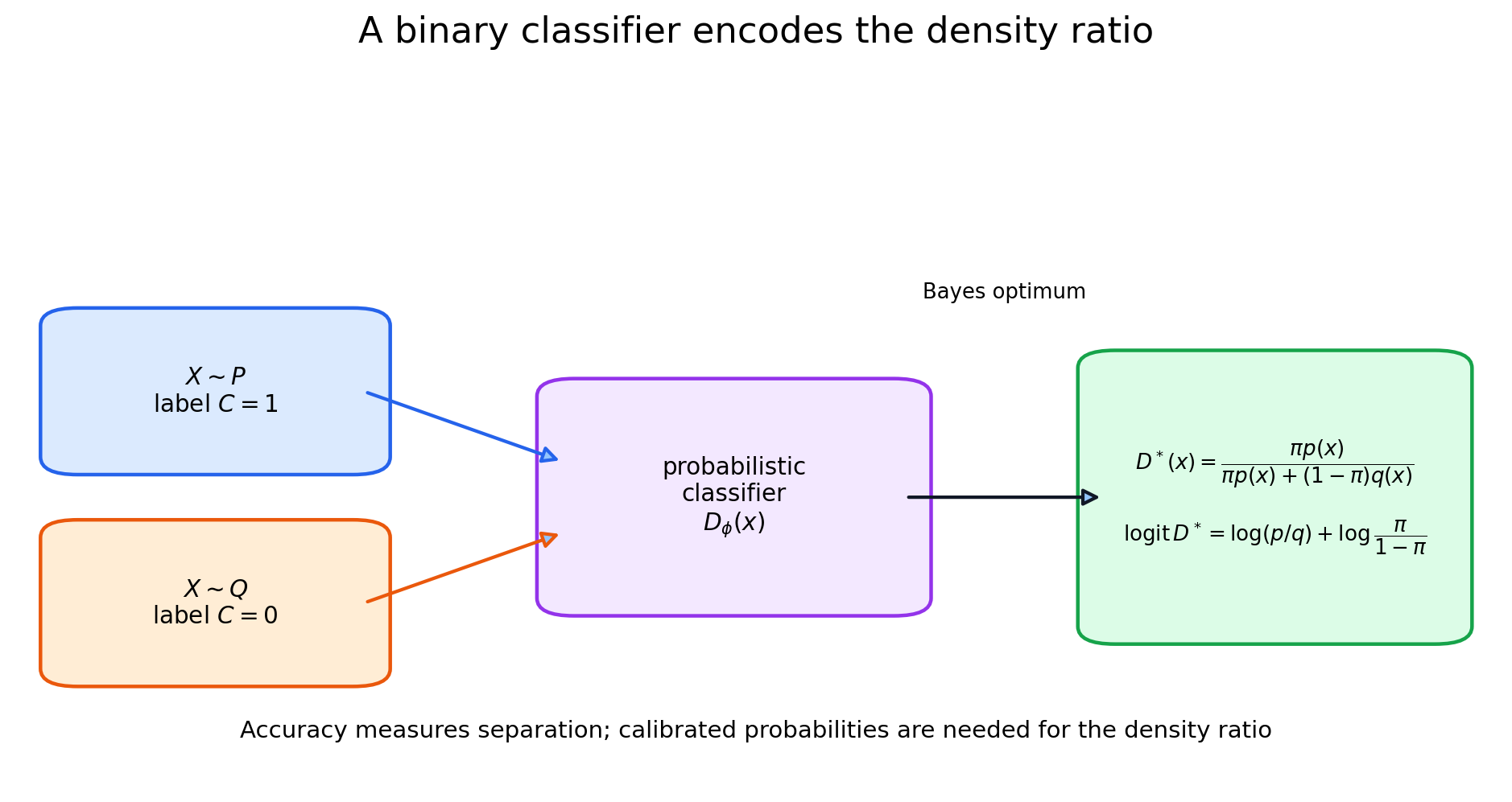
Bayes' rule gives the optimal probabilistic classifier:

$$D^*(x) = \Pr(C=1\mid X=x) = \frac{\pi p(x)} {\pi p(x)+(1-\pi)q(x)}.$$

Taking odds,

$$\frac{D^*(x)}{1-D^*(x)} = \frac{\pi p(x)}{(1-\pi)q(x)},$$

and hence

$$\boxed{ \operatorname{logit}D^*(x) = \log\frac{p(x)}{q(x)} + \log\frac{\pi}{1-\pi} }.$$

For equal class priors, the prior-odds term disappears:

$$\operatorname{logit}D^*(x) = \log\frac{p(x)}{q(x)}.$$

In the two-point example from Section 11.1,

$$D^*(a)=0.8, \qquad D^*(b)=0.2,$$

so

$$\operatorname{logit}D^*(a)=\log4, \qquad \operatorname{logit}D^*(b)=-\log4.$$

The ideal classifier recovers exactly the log-ratio required by KL and many related divergences.

This is a central tool in likelihood-free inference: instead of estimating two densities separately, we estimate one function that distinguishes their samples.

Two tasks must still be separated:

• source classification requires the correct decision or ranking;
• density-ratio estimation also requires calibrated probabilities.

With nearly separable classes, accuracy can be perfect while logits are arbitrarily overconfident. High classification accuracy confirms that the samples are distinguishable, but it does not by itself provide an accurate numerical estimate of $p/q$.

11.5. Variational form: making a discrepancy trainable

Classification gave one route to a density ratio. We now derive a mechanism that works for the entire family of f-divergences.

From Fenchel's inequality to a lower bound

For convex $f$, define the convex conjugate

$$\boxed{ f^*(s) = \sup_{t>0}\{st-f(t)\} }.$$

The definition implies Fenchel's inequality,

$$f(t)\ge st-f^*(s),$$

for every admissible $s$. Choose $s=T(x)$ pointwise and set $t=p(x)/q(x)$:

$$f\!\left(\frac pq\right) \ge T\frac pq-f^*(T).$$

Multiply by $q$ and integrate:

$$\begin{aligned} D_f(P\|Q) &= \mathbb E_Q f\!\left(\frac pq\right)\\ &\ge \mathbb E_Q\!\left[T\frac pq-f^*(T)\right]\\ &= \mathbb E_P[T] - \mathbb E_Q[f^*(T)]. \end{aligned}$$

Thus every admissible function $T$ gives a lower bound:

$$\boxed{ \mathbb E_P[T] - \mathbb E_Q[f^*(T)] \le D_f(P\|Q) }.$$

With a sufficiently rich function class and the appropriate regularity conditions, taking the supremum yields

$$\boxed{ D_f(P\|Q) = \sup_T \left\{ \mathbb E_P[T(X)] - \mathbb E_Q[f^*(T(X))] \right\} }.$$

For differentiable strictly convex $f$, the pointwise optimizer satisfies

$$\boxed{ T^*(x) = f'\!\left(\frac{p(x)}{q(x)}\right) }.$$

If $f'$ is invertible, the ideal critic recovers the density ratio:

$$\frac{p(x)}{q(x)} = (f')^{-1}(T^*(x)).$$

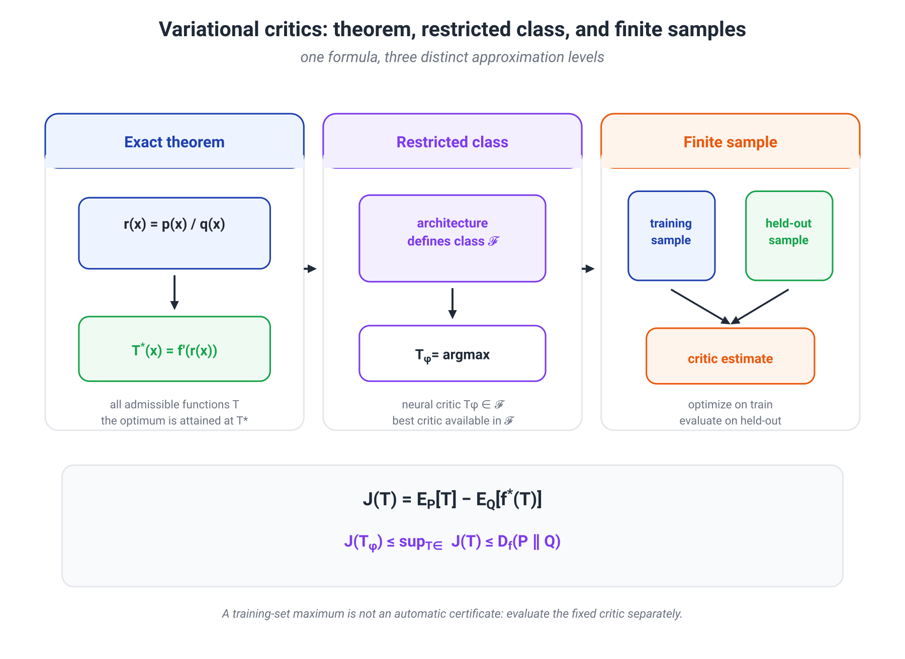
The critic's role is now exact. It need not output a class probability; in general, it learns the transformation of the density ratio selected by $f$.

From the theorem to a neural training run

Let $\mathcal T$ be a restricted critic class, such as a fixed neural architecture. Then

$$\sup_{T\in\mathcal T} \left\{ \mathbb E_PT- \mathbb E_Qf^*(T) \right\} \le D_f(P\|Q).$$

A practical run adds three more approximations:

1. population expectations are replaced by finite-sample averages;
2. optimization does not find the best critic even within $\mathcal T$;
3. the same data are often used both to fit the critic and to report its value.

The third point is especially important. For a fixed $T$, the population objective is a lower bound. The maximum empirical objective over a flexible class can overfit and exceed the population divergence. A sound protocol separates critic training from held-out evaluation and includes a permutation baseline.

KL: the NWJ and Donsker–Varadhan forms

For forward KL, take

$$f(t)=t\log t.$$

Its conjugate is

$$f^*(s)=e^{s-1}.$$

The general formula becomes

$$\boxed{ D_{\mathrm{KL}}(P\|Q) = \sup_T \left\{ \mathbb E_P[T] - \mathbb E_Q[e^{T-1}] \right\} }.$$

In the mutual-information estimation literature, this is often called the Nguyen–Wainwright–Jordan, or NWJ, form. Its optimal critic is

$$T^*(x)=1+\log\frac{p(x)}{q(x)}.$$

Another exact representation is Donsker–Varadhan:

$$\boxed{ D_{\mathrm{KL}}(P\|Q) = \sup_G \left\{ \mathbb E_P[G] - \log\mathbb E_Q[e^G] \right\} }.$$

The relationship is easier to derive than to memorize. Substitute $T=G+c$ into the NWJ objective:

$$\mathbb E_P[G]+c - e^{c-1}\mathbb E_Q[e^G].$$

The optimum over the free shift $c$ is

$$c^*=1-\log\mathbb E_Q[e^G].$$

Substitution leaves the DV objective. Consequently, the optimal DV critic is defined only up to an additive constant:

$$G^*(x) = \log\frac{p(x)}{q(x)}+\text{const}.$$

Both formulas are exact at the population level, but their finite-sample estimators behave differently. The exponential and the logarithm of a normalization average make the DV objective particularly sensitive to rare large critic values.

11.6. GAN and f-GAN

The adversarial game now stops looking like an isolated trick. It is one way to fit a variational critic while simultaneously moving the distribution being compared with the data.

The original minimax GAN

Goodfellow et al. use the objective

$$\max_D \left\{ \mathbb E_{P_{\mathrm{data}}}[\log D(X)] + \mathbb E_{Q_\theta}[\log(1-D(X))] \right\}.$$

For a fixed generator, the pointwise optimum is

$$D^*(x) = \frac{p_{\mathrm{data}}(x)} {p_{\mathrm{data}}(x)+q_\theta(x)}.$$

Let

$$M=\frac12(P_{\mathrm{data}}+Q_\theta).$$

Substituting the optimal discriminator gives

$$\boxed{ \max_D V(D,Q_\theta) = -\log4 + 2D_{\mathrm{JS}}(P_{\mathrm{data}},Q_\theta) }.$$

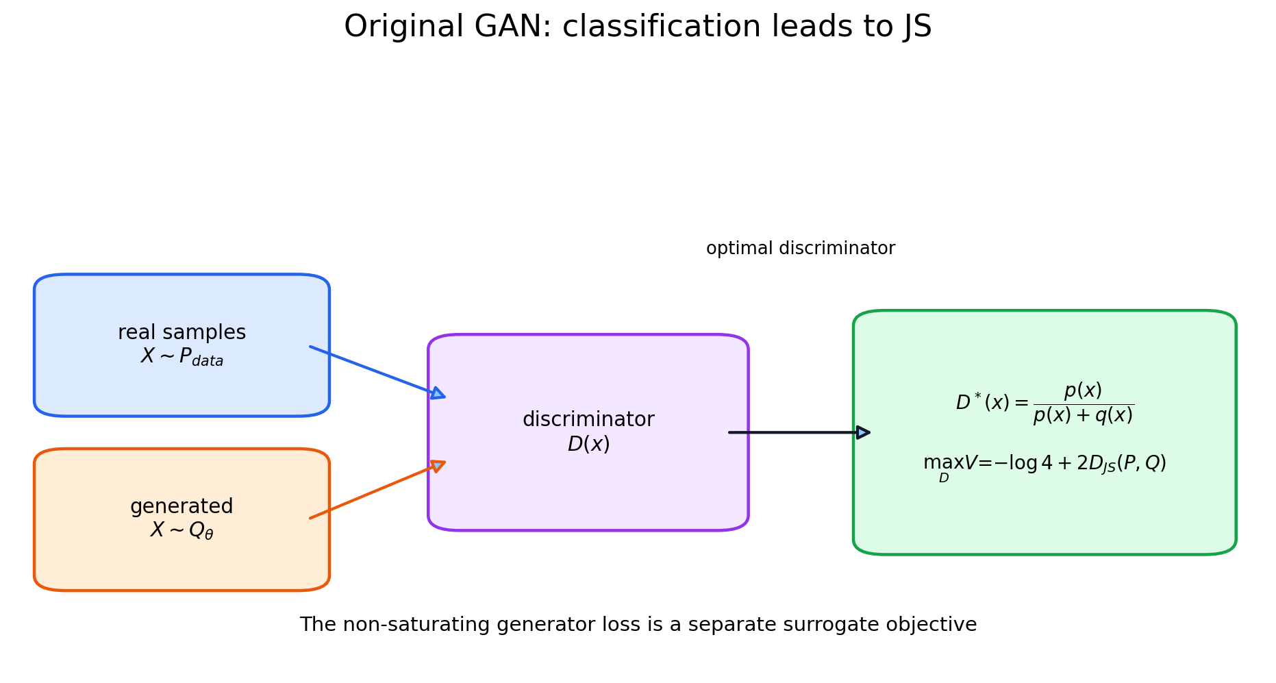
This is a strong and exact statement: the idealized minimax game with an optimal discriminator compares the data and generator distributions through Jensen–Shannon divergence.

Actual training solves the inner problem only approximately. The generator belongs to a restricted parametric family, and the commonly used non-saturating loss

$$-\mathbb E_{Q_\theta}\log D(X)$$

replaces the original saturating objective to provide a stronger early gradient. The desired fixed point $P_{\mathrm{data}}=Q_\theta$ is preserved, but an individual generator update is no longer literal gradient descent on exact JS.

f-GAN

The general variational representation replaces JS by another f-divergence:

$$\boxed{ \min_\theta\max_\phi \left\{ \mathbb E_{P_{\mathrm{data}}}[T_\phi(X)] - \mathbb E_{Q_\theta}[f^*(T_\phi(X))] \right\} }.$$

If the critic class is sufficiently rich and the inner maximum is solved, the inner value equals

$$D_f(P_{\mathrm{data}}\|Q_\theta).$$

Some conjugates $f^*$ have restricted domains. f-GAN therefore maps an unconstrained network output $V_\phi$ through

$$T_\phi(x)=g_f(V_\phi(x))$$

so that

$$T_\phi(x)\in\operatorname{dom}f^*.$$

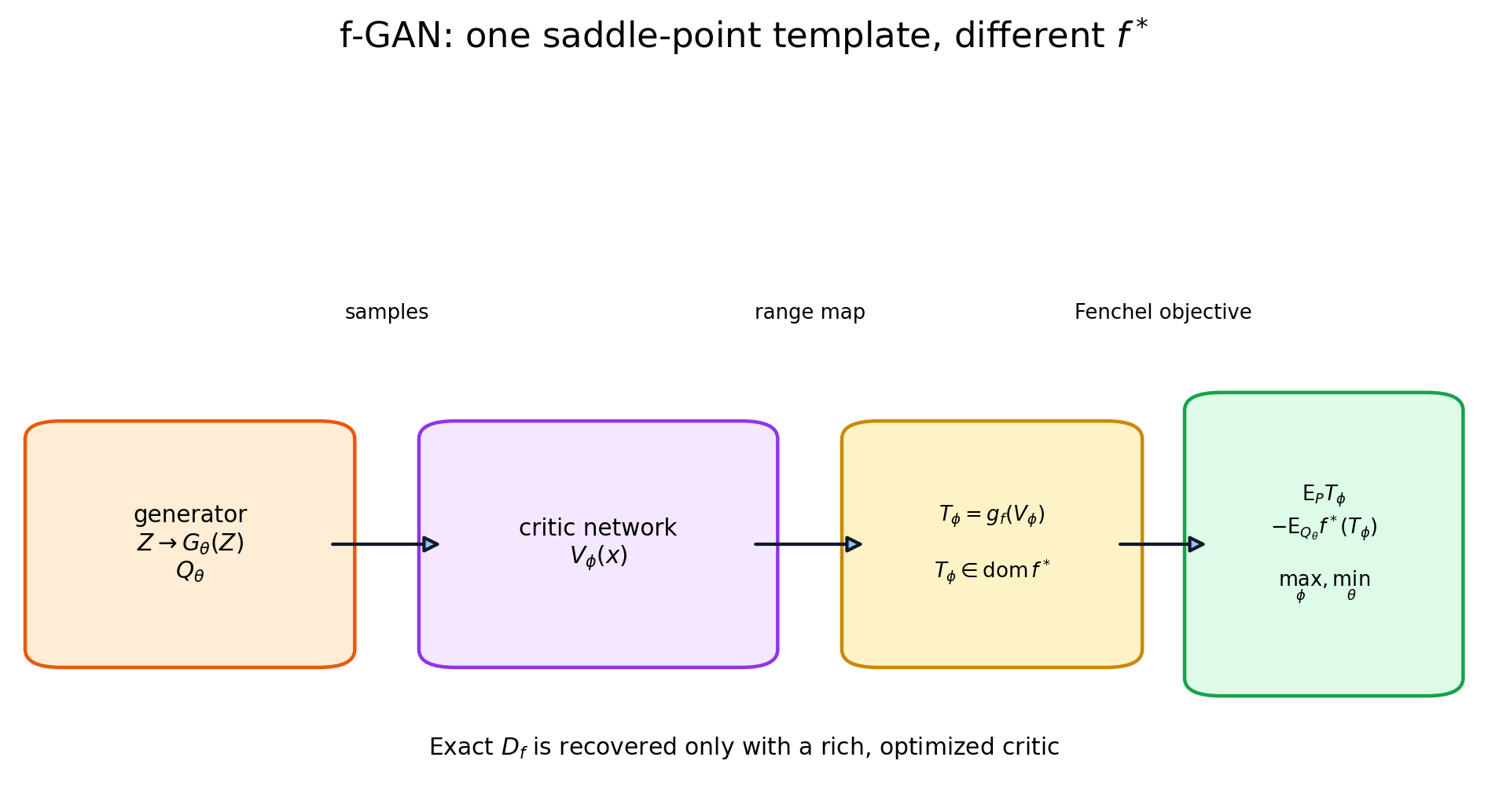
The choice of $f$ changes several parts of the problem:

• the projection selected within a restricted generator family;
• the shape and curvature of the critic loss;
• the admissible critic output range;
• sensitivity to different density-ratio regimes;
• the bias–variance tradeoff of the estimator.

It is useful to separate two levels. In the idealized population problem, the divergence defines the destination. In an actual GAN, saddle-point dynamics determine whether training approaches it. Mode collapse, oscillations, and instability depend not only on $f$, but also on architecture, regularization, relative learning rates, and the generator's surrogate loss.

11.7. MINE and InfoNCE

Mutual information is already a distribution-comparison problem:

$$I(X;Y) = D_{\mathrm{KL}} (P_{XY}\|P_X\otimes P_Y).$$

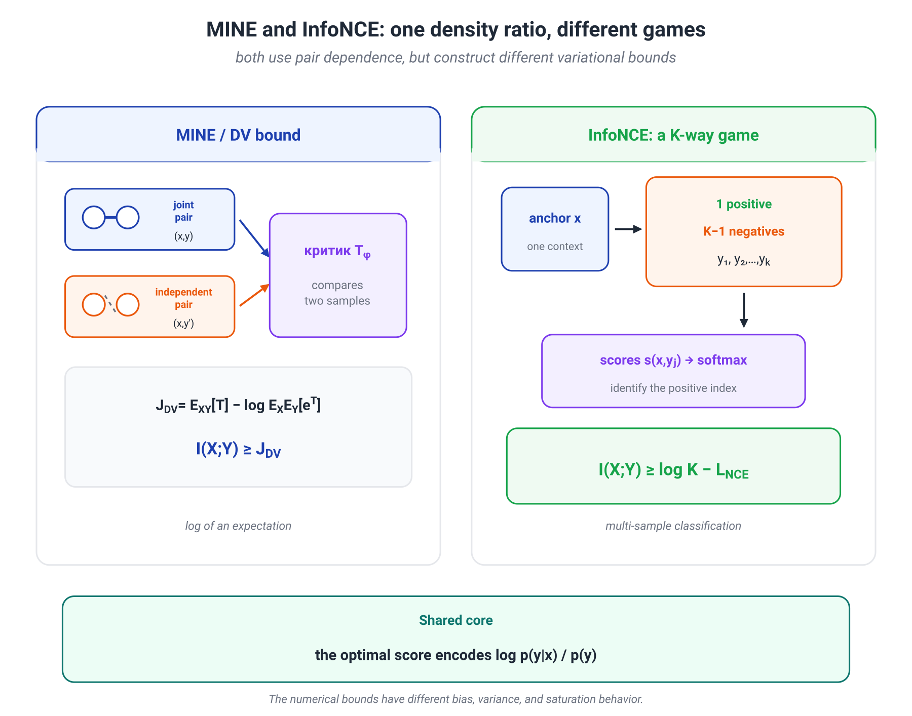
The joint distribution supplies genuine pairs $(X,Y)$. The product of marginals supplies independently assembled pairs. Estimating MI can therefore be turned into distinguishing associated pairs from shuffled ones.

MINE: a DV critic for joint versus product

MINE substitutes these distributions into the Donsker–Varadhan representation:

$$\boxed{ I(X;Y) \ge \mathbb E_{P_{XY}}[T_\phi(X,Y)] - \log \mathbb E_{P_X\otimes P_Y} [e^{T_\phi(X,Y)}] }.$$

Positive pairs come from the joint distribution. Samples from the product of marginals can be formed by independently resampling $X$ and $Y$; shuffling $Y$ within a minibatch is a common approximation.

The population expression is simple, but finite-sample estimation is difficult because of the exponential. Rare large critic values can dominate the normalization term and create high variance. The original MINE procedure used a moving average to stabilize the gradient of that term.

A useful protocol separates three steps:

1. train the critic on training pairs;
2. evaluate the objective on held-out pairs;
3. use a permutation experiment to verify that the estimate returns to its null baseline when dependence is destroyed.

InfoNCE: choosing the positive candidate

InfoNCE uses a different game. For each $X$, one candidate $Y_1$ is drawn from $P(Y\mid X)$, while

$$Y_2,\ldots,Y_K \overset{\mathrm{iid}}{\sim}P_Y$$

are negative candidates. The critic must identify the positive pair:

$$\mathcal L_{\mathrm{NCE}} = - \mathbb E \log \frac{e^{s(X,Y_1)}} {\sum_{j=1}^{K}e^{s(X,Y_j)}}.$$

Under this sampling scheme,

$$\boxed{ I(X;Y) \ge \log K- \mathcal L_{\mathrm{NCE}} }.$$

The optimal score has the form

$$s^*(x,y) = \log\frac{p(y\mid x)}{p(y)}+c(x),$$

so the same density ratio appears again.

For example, $K=32$ and a loss of $1.2$ nats give

$$\log32-1.2 \approx 2.266\ \text{nats} \approx 3.27\ \text{bits}.$$

This is an MI lower bound under the specified sampling scheme, not a standalone measurement of all information in the representation.

One density ratio, different sample objectives

MINE and InfoNCE converge toward related optimal score functions, but they construct different variational problems:

• MINE uses the DV functional with an exponential expectation;
• InfoNCE solves a $K$-way positive-candidate classification problem.

Calling InfoNCE “MINE with a small bias” therefore hides the actual distinction.

InfoNCE has an explicit ceiling:

$$\log K-\mathcal L_{\mathrm{NCE}} \le \log K.$$

Increasing $K$ raises the ceiling and can tighten the bound under an ideal critic. Representation learning, however, depends on more than the reported bound: false negatives, augmentations, compute, and optimization difficulty can all change downstream quality.

This leads to an important distinction:

A variational bound can be a useful training signal even when its numerical value is a poor absolute MI meter.

When true MI is large, neural lower bounds face a bias–variance tradeoff. More broadly, without additional assumptions, a distribution-free high-confidence lower bound from $N$ observations cannot reliably grow much faster than order $\log N$. This limits statistical certification; it does not forbid using a contrastive objective as a learning signal.

11.8. Integral probability metrics: Wasserstein distance and MMD

f-divergences quantify probability reweighting. Some tasks must also distinguish a nearby mismatch from a distant one.

Two moving point masses

Let

$$P=\delta_0, \qquad Q_\theta=\delta_\theta.$$

For every $\theta\ne0$, the supports are disjoint, so

$$D_{\mathrm{JS}}(P,Q_\theta)=\log2, \qquad \operatorname{TV}(P,Q_\theta)=1,$$

and both KL directions are infinite. These values do not change as $\theta$ moves from $10^{-3}$ to $10^3$.

Wasserstein-1 does see the displacement:

$$\boxed{ W_1(P,Q_\theta)=|\theta| }.$$

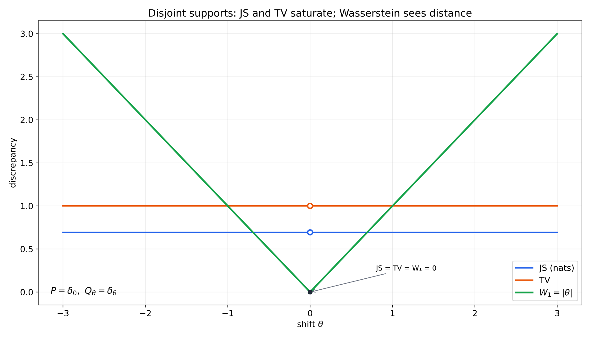
The example motivates a different language: rather than starting from a density ratio, start from a class of test functions that is sensitive to the relevant geometry.

Integral probability metrics

For a symmetric function class $\mathcal F$, define

$$\boxed{ \operatorname{IPM}_{\mathcal F}(P,Q) = \sup_{h\in\mathcal F} \left| \mathbb E_P[h(X)]- \mathbb E_Q[h(X)] \right| }.$$

The class $\mathcal F$ determines which discrepancies the critic can observe. A class that is too simple misses differences; a very rich class is harder to estimate and optimize.

Wasserstein-1

Let the sample space carry a metric $d$, and assume $P$ and $Q$ have finite first moments. For the class of all 1-Lipschitz functions, Kantorovich–Rubinstein duality gives

$$\boxed{ W_1(P,Q) = \sup_{\|h\|_{\mathrm{Lip}}\le1} \left( \mathbb E_Ph- \mathbb E_Qh \right) }.$$

The same quantity has the transport form

$$\boxed{ W_1(P,Q) = \inf_{\gamma\in\Pi(P,Q)} \mathbb E_{(X,Y)\sim\gamma}[d(X,Y)] }.$$

Here $\Pi(P,Q)$ is the set of couplings with marginals $P$ and $Q$. The first formula describes the best 1-Lipschitz critic; the second describes the minimum average cost of transporting probability mass.

Wasserstein distance depends on the ground metric. Multiplying all coordinates by one hundred changes the transport cost. That is not a defect: the metric states which displacements the problem considers small.

WGAN

Wasserstein GAN trains a critic with the objective

$$\max_{\|h_\phi\|_{\mathrm{Lip}}\le1} \left\{ \mathbb E_{P_{\mathrm{data}}}[h_\phi(X)] - \mathbb E_{Q_\theta}[h_\phi(X)] \right\}.$$

The inner maximum equals $W_1$ in the ideal problem. The main engineering challenge is enforcing the Lipschitz condition.

The original WGAN used weight clipping. WGAN-GP replaced clipping with the penalty

$$\lambda \mathbb E_{\widehat X} \left( \|\nabla_{\widehat x}h_\phi(\widehat X)\|_2-1 \right)^2$$

on interpolated points. This often gives a better-behaved training problem, but it is not a global certificate that the neural critic is 1-Lipschitz everywhere.

The positive result of WGAN is not a promise that every run converges. It is a population discrepancy with more informative geometry for nearby disjoint supports. Practical performance still depends on the critic class, the Lipschitz-control mechanism, and optimization dynamics.

MMD: a kernel-defined critic class

If $\mathcal F$ is the unit ball of a reproducing-kernel Hilbert space $\mathcal H_k$, the IPM becomes maximum mean discrepancy:

$$\operatorname{MMD}_k(P,Q) = \sup_{\|h\|_{\mathcal H_k}\le1} \left| \mathbb E_Ph- \mathbb E_Qh \right|.$$

Its square can be computed without an inner neural optimization:

$$\boxed{ \begin{aligned} \operatorname{MMD}_k^2(P,Q) &= \mathbb E_{X,X'\sim P}k(X,X')\\ &\quad- 2\mathbb E_{X\sim P,Y\sim Q}k(X,Y)\\ &\quad+ \mathbb E_{Y,Y'\sim Q}k(Y,Y'). \end{aligned} }$$

For a characteristic kernel, MMD$=0$ if and only if $P=Q$. The Gaussian kernel

$$k_\sigma(x,y) = \exp\left(-\frac{\|x-y\|^2}{2\sigma^2}\right)$$

is characteristic on Euclidean space. Its bandwidth $\sigma$ determines the scale of visible differences: an overly small bandwidth sees only local coincidences, while an overly large one smooths away structure.

MMD is useful for two-sample testing and shift detection. Its empirical estimate is built from pairwise kernel evaluations and requires no adversarial inner loop. The tradeoff is that the kernel must encode a meaningful notion of similarity, and the naive estimator has quadratic sample complexity in time.

The families overlap

f-divergences and IPMs are not disjoint boxes. Total variation has both representations:

$$\operatorname{TV}(P,Q) = \frac12\int|p-q|$$

and

$$\operatorname{TV}(P,Q) = \sup_{0\le h\le1} \left| \mathbb E_Ph- \mathbb E_Qh \right|.$$

The useful distinction is the mechanism:

• an f-divergence obtains its geometry from the density ratio and the function $f$;
• an IPM obtains its geometry from the test-function class $\mathcal F$.

11.9. Choosing a discrepancy in practice

There is no universally best discrepancy. The choice begins with what the system can observe and what it should count as an error.

Four questions provide a useful decision procedure.

1. What can be computed?

Are $p(x)$ and $q(x)$ available, or only samples? Can gradients flow through the generator? Does the problem naturally provide positive and negative pairs?

2. Which error matters?

Should the objective heavily penalize missing mass, extra mass, geometric displacement, selected moments, or any distinction visible to a chosen test-function class?

3. What is actually being optimized?

An exact discrepancy, a variational lower bound, a finite-sample estimator, and a generator surrogate are different objects. They may share an ideal optimum while having different training trajectories and statistical behavior.

4. How will the result be checked?

A critic value should be complemented by independent evidence: a held-out objective, a downstream metric, domain-specific inspection, a permutation baseline, or sensitivity across kernels and critic classes.

The practical principle is more useful than a slogan about the “best distance”:

A good discrepancy aligns the meaning of error, the available estimator, and the geometry of the model's sample space.

11.10. Mathematical deepening: general measures and exact duality

Optional on a first pass. This section makes precise the places where the main route assumed densities with $P\ll Q$.

General f-divergence and the singular part

Let $P$ and $Q$ be dominated by a measure $\mu$:

$$p=\frac{dP}{d\mu}, \qquad q=\frac{dQ}{d\mu}.$$

Define the boundary values

$$f(0)=\lim_{t\downarrow0}f(t), \qquad f'_\infty = \lim_{t\to\infty}\frac{f(t)}t.$$

The extended f-divergence is

$$\boxed{ D_f(P\|Q) = \int_{\{q>0\}} q f\!\left(\frac pq\right)d\mu + f'_\infty P\{q=0\} }.$$

The value does not depend on the chosen dominating measure. If $P\perp Q$, then

$$D_f(P\|Q)=f(0)+f'_\infty.$$

This immediately yields the boundary values:

• TV: $1$;
• squared Hellinger distance in our normalization: $1$;
• JS: $\log2$;
• forward KL and Pearson $\chi^2$: $+\infty$.

Joint convexity

The two-variable function

$$\psi(p,q)=qf(p/q)$$

is the perspective of the convex function $f$ and is jointly convex in $(p,q)$. Integrating gives, for $0\le\lambda\le1$,

$$\begin{aligned} &D_f\bigl(\lambda P_1+(1-\lambda)P_2 \,\|\, \lambda Q_1+(1-\lambda)Q_2\bigr)\\ &\qquad\le \lambda D_f(P_1\|Q_1) +(1-\lambda)D_f(P_2\|Q_2). \end{aligned}$$

This formalizes a simple idea: mixing two comparison problems cannot create more discrepancy than their average pre-mixture score.

When the variational supremum is exact

The identity

$$D_f(P\|Q) = \sup_T \left\{ \mathbb E_PT- \mathbb E_Qf^*(T) \right\}$$

requires convexity and lower semicontinuity of $f$, a correct domain for $f^*$, a sufficiently rich measurable function class, and conditions that justify the pointwise optimizer and the interchange of integration with the supremum.

For differentiable $f$,

$$T^*(x)=f'\!\left(\frac{p(x)}{q(x)}\right).$$

For nondifferentiable generators such as TV, the derivative is replaced by a subgradient condition:

$$T^*(x) \in \partial f\!\left(\frac{p(x)}{q(x)}\right).$$

A neural critic class is almost always smaller than the full measurable function class. The optimized expression in code should therefore be called a variational lower bound unless tightness has been established for the chosen architecture and procedure.

11.12. Conclusion

KL led us into this module, but the resulting picture is broader than one divergence.

f-divergences collect a large class of discrepancies into one expression:

$$D_f(P\|Q) = \mathbb E_Q f\!\left(\frac pq\right).$$

The function $f$ determines how different density-ratio errors are priced. Data processing explains why a fixed transformation cannot increase population distinguishability, while saturation on disjoint supports shows where a density-ratio view loses external geometry.

Fenchel duality turns an inaccessible discrepancy into a trainable problem:

$$D_f(P\|Q) = \sup_T \left\{ \mathbb E_PT- \mathbb E_Qf^*(T) \right\}.$$

Ideally, the critic recovers a transformation of $p/q$. In a real run, it operates in a restricted class, on finite data, and with finite optimization. A critic value is therefore useful to the extent that this protocol is stated clearly.

The same mechanism connects several methods that initially look unrelated:

• a probabilistic classifier estimates a log density ratio;
• the original minimax GAN is linked to JS under an optimal discriminator;
• f-GAN changes $f$ and the critic's conjugate loss;
• MINE compares joint and shuffled pairs through the DV representation;
• InfoNCE solves a multi-candidate classification problem whose optimal score contains the same ratio.

When distances between points matter in their own right, the language changes. Wasserstein distance uses transport cost in a ground metric, whereas MMD measures distinguishability by a kernel-defined test-function class.

The engineering conclusion is:

Choose a discrepancy by the error it makes expensive, the estimator you can actually run, and the geometry your task needs—not by the reputation of its name.

Module 12 will use the same variational apparatus in a different role. KL will measure how far a data-dependent posterior moves from a prior, and PAC-Bayes will turn that cost into a generalization bound.

Primary references

1. X. Nguyen, M. Wainwright, M. Jordan, Estimating Divergence Functionals and the Likelihood Ratio by Convex Risk Minimization, 2010.
2. S. Nowozin, B. Cseke, R. Tomioka, f-GAN: Training Generative Neural Samplers using Variational Divergence Minimization, 2016.
3. I. Goodfellow et al., Generative Adversarial Nets, 2014.
4. M. Belghazi et al., MINE: Mutual Information Neural Estimation, 2018.
5. A. van den Oord, Y. Li, O. Vinyals, Representation Learning with Contrastive Predictive Coding, 2018.
6. B. Poole et al., On Variational Bounds of Mutual Information, 2019.
7. D. McAllester, K. Stratos, Formal Limitations on the Measurement of Mutual Information, 2020.
8. M. Arjovsky, S. Chintala, L. Bottou, Wasserstein GAN, 2017.
9. I. Gulrajani et al., Improved Training of Wasserstein GANs, 2017.
10. A. Gretton et al., A Kernel Two-Sample Test, 2012.