Module 14. Computer Vision Through Information Theory
How to read this module. This is a bonus module for readers working with images, multimodal models, and deployed computer-vision systems. The main route is Sections 14.1–14.8. It begins with the most literal connection to information theory—compressing an image into an actual bitstream—and then moves to perceptual quality, diffusion models, CLIP, self-supervised visual representation learning, and compression of the model itself. Section 14.9 is optional mathematical deepening on exact rate accounting in a hyperprior codec and Gaussian denoising identities.
14.1. Why computer vision is a useful testbed for information theory
Consider an ordinary RGB image with eight bits per channel. In raw form it occupies
bits, exactly MiB. Yet the same image can play several very different roles inside a vision system.
- It can be stored or transmitted, spending bits while tolerating controlled distortion.
- It can be observed through noise and restored as accurately as possible.
- It can be mapped to a compact representation for classification, retrieval, segmentation, or control.
- Finally, the model itself must be deployed under limits on memory, bandwidth, latency, and energy.
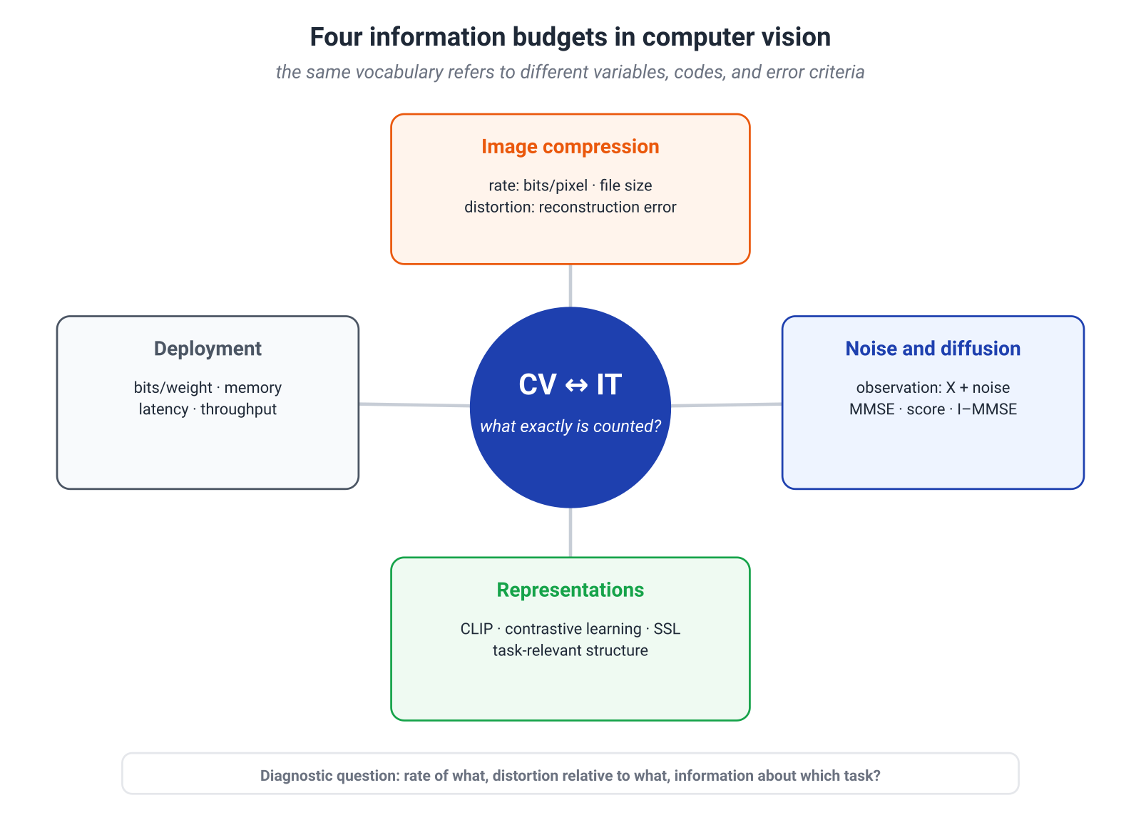
All four settings use words such as compression, information, noise, and bottleneck. Their mathematical meanings are not the same.
In a learned image codec, the connection to Shannon is operational: there is a source, a quantized symbol, a probabilistic entropy model, a coder, and a file whose size can be counted. In diffusion, exact Gaussian identities connect posterior means, scores, and mutual information, but those identities do not specify the complete architecture or sampling algorithm. In CLIP and self-supervised learning, information-theoretic quantities help interpret the training game, but they do not turn every encoder into an optimal Information Bottleneck. In weight quantization, the rate–distortion analogy becomes useful only after we state what rate is physically measured and what error is treated as distortion.
This scale of exactness is more useful than a catalog of methods:
| Setting | What is defined precisely | What the engineer must still choose |
|---|---|---|
| Image compression | bitstream, decoder, distortion measure | architecture, entropy model, latency |
| Denoising and diffusion | Gaussian channel, MSE optimum, score identities | noise schedule, parameterization, sampler |
| CLIP and SSL | training game and surrogate loss | augmentations, negatives, downstream task |
| Model compression | numerical format and resource budget | the relevant functional distortion |
The main habit of this module is simple:
Before invoking information, name the random variables, the code or observation, and the criterion by which error is paid.
With that habit, many ambitious analogies become both narrower and more useful.
14.2. Learned image compression: entropy models and actual bitstreams
We begin where the connection to information theory can be checked literally: store an image, then reconstruct it from the resulting file.
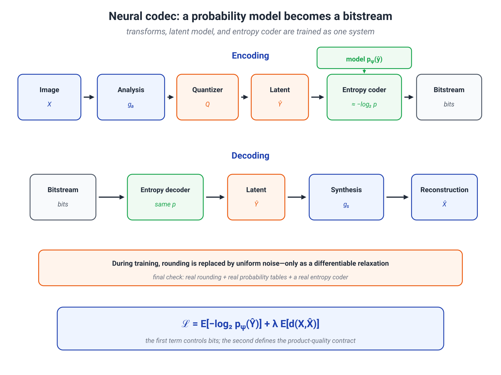
A learned codec constructs a latent representation
quantizes it,
and reconstructs the image,
Here is the analysis transform and is the synthesis transform. Their roles resemble the forward and inverse transforms of a classical transform codec, but both are learned from data.
A latent tensor is not yet a compressed file. To emit a bitstream, the coder needs probabilities for its discrete symbols. Suppose the entropy model assigns
to a particular latent. An arithmetic or range coder can then transmit it in approximately
bits, plus finite overhead from termination, headers, and finite-precision arithmetic.
It is worth reading the formula literally. If the average model bill is bits per pixel, then a image requires an idealized
bits, or KiB. This is no longer a metaphor about a “compact representation.” It is a number that can be compared with the physical file.
The rate–distortion objective
A standard training objective is
The multiplier sets the exchange rate between bits and reconstruction quality. Different values of produce different operating points on an empirical rate–distortion curve.
This is where the phrase “the network learns to compress” becomes mathematically concrete. The probabilistic model does not merely regularize the latent: its logarithmic score drives the entropy coder. Early end-to-end learned codecs optimized the analysis transform, the entropy model, and the synthesis transform in exactly this joint setup. (Ballé, Laparra & Simoncelli, 2017)
Training through nondifferentiable quantization
Rounding is convenient for a file and inconvenient for a gradient. A common relaxation replaces it during training with additive uniform noise:
The continuous density of is trained so that its mass over a unit quantization interval approximates the probability of the eventual discrete symbol. This provides a smooth surrogate objective.
But a surrogate remains a surrogate. Final evaluation should use real rounding, the actual probability tables, and a real entropy coder. The continuous objective may predict the rate well without matching every emitted file down to the last bit.
Hyperpriors: sometimes it is worth describing the context first
Compare a smooth sky patch with dense foliage. The main latent tensor has the same format in both cases, but the expected local scale and variability of its coefficients differ. A single fully factorized model has to describe both regimes with one rule.
A hyperprior transmits an auxiliary latent
which helps the decoder predict parameters of the main latent distribution:
The total model rate is
The intuition is straightforward: spend a few bits describing the local regime, then code a large collection of primary symbols more accurately. The scale hyperprior was introduced precisely as learned side information about spatially varying latent statistics. (Ballé et al., 2018)
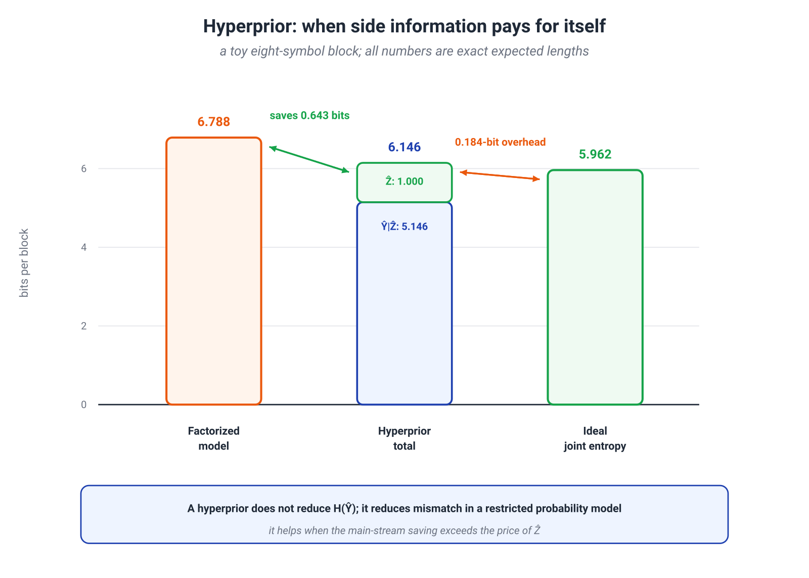
There is an easy overstatement to avoid. The chain rule does not say that introducing magically lowers the fundamental entropy of :
The practical gain is a comparison between restricted model classes. A simple factorized prior may badly miss dependencies in , while a conditional model with a hyperprior may reduce mismatch enough that the savings on the main stream exceed the cost of . Section 14.9 writes this balance as an exact KL decomposition.
Context models: fewer bits, more sequential dependence
Another way to improve the entropy model is to use already decoded symbols:
This context can lower cross-entropy by exploiting local dependencies. Hierarchical and autoregressive priors are complementary; models combining them demonstrated exactly that. (Minnen, Ballé & Toderici, 2018)
The price is sequential decoding: symbol depends on earlier symbols. A better probability model is therefore not automatically a better deployed codec. Modern systems explicitly trade modeling accuracy against parallelism and latency.
A serious codec comparison should report at least:
- actual bits per pixel;
- the distortion measure;
- encoding and decoding latency;
- peak memory;
- model and side-information cost;
- bitstream compatibility and reproducibility.
Information theory gives the core objective. Engineering determines the price of realizing it.
14.3. Distortion and perceptual quality
A rate–distortion problem must choose
In computer vision, that choice is unusually visible: it decides what the codec or restoration system counts as an error.
Suppose two fine textures are equally plausible given a noisy observation. Squared error prefers their conditional mean. Mathematically this is correct—the posterior mean minimizes MSE. Visually, the average of two textures can be blurry and resemble neither one.
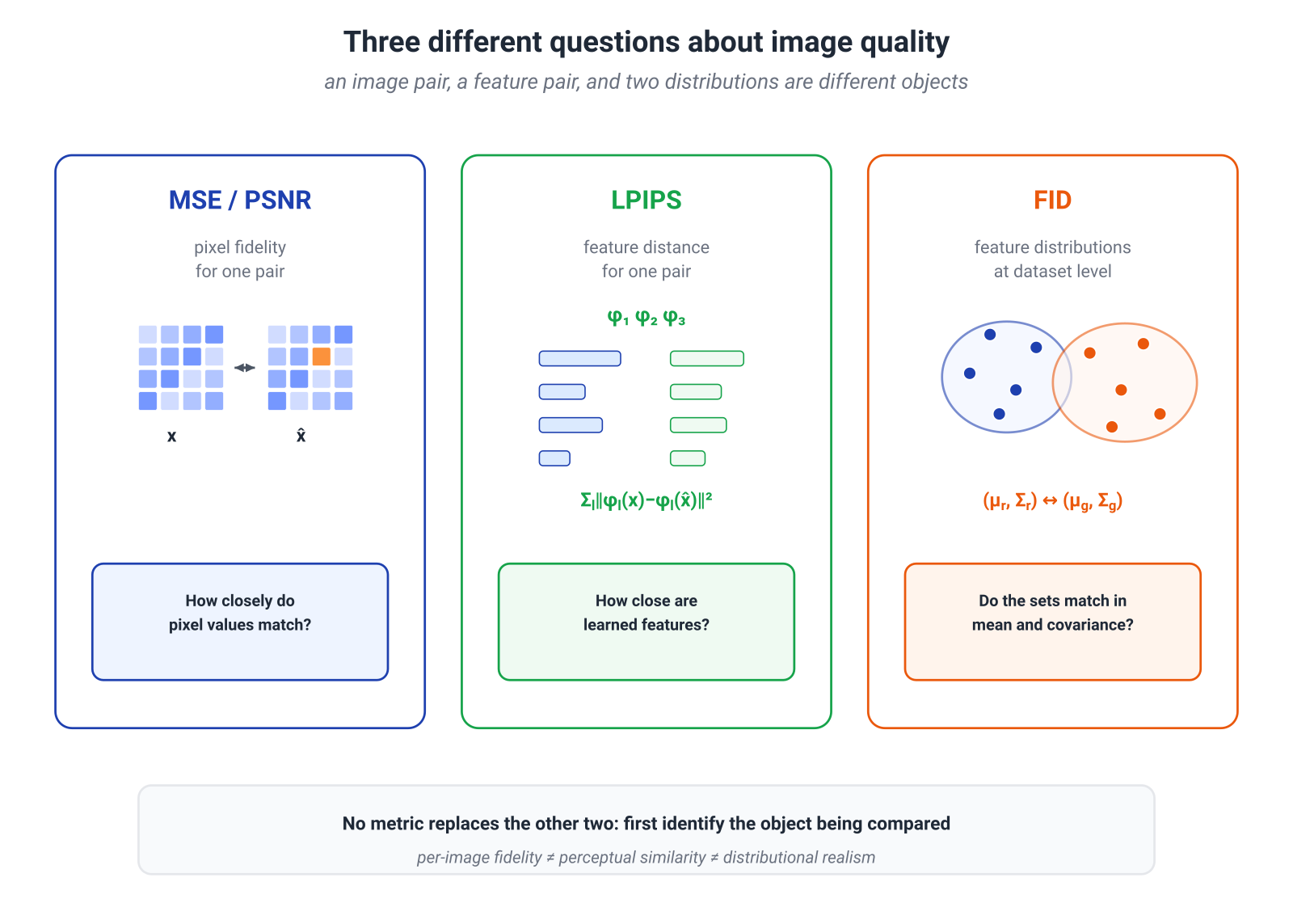
This separates three questions.
- How close is the reconstruction to this particular source image?
- How similar is the pair in a learned feature space?
- How close is the distribution of reconstructions to the distribution of natural images?
A single metric rarely answers all three.
MSE and PSNR: pixel fidelity
Mean squared error is
For a fixed pixel range, PSNR is a monotone transformation of MSE. These measures are stable and interpretable when numerical pixel fidelity matters.
Their limitation is not that they are “bad,” but that they answer a narrow question. In medical imaging, astronomy, or remote sensing, pixel fidelity may be more important than visual plausibility. For a social-media thumbnail, the product objective may be different.
LPIPS: a feature-space distance for a pair of images
LPIPS compares normalized features from several layers of a deep network. Schematically,
Its weights were calibrated on human perceptual judgments, and on the corresponding benchmarks it aligned with those judgments better than several traditional pixel metrics. (Zhang et al., 2018)
The object must be named correctly: LPIPS is a distance between a particular image pair in a chosen feature space. It is not MMD, not an f-divergence, and not a comparison between two image distributions.
FID: comparing distributions in feature space
A generator or generative codec raises a different question: does the set of reconstructions look like a sample from the real-data distribution?
FID approximates the two Inception-feature distributions by Gaussians and computes their squared distance:
This is a dataset-level statistic. A good FID does not guarantee that a particular reconstruction preserved a particular source detail. Conversely, a low MSE for individual pairs does not guarantee that the output distribution looks realistic. FID was introduced by Heusel et al. (2017).
Rate–distortion–perception
Blau and Michaeli added an explicit distributional constraint to the classical distortion constraint:
subject to
With no perception constraint, this reduces to ordinary rate–distortion theory. If reconstructions must be both faithful to individual inputs and statistically realistic, the achievable region generally shrinks. Better perception must be paid for in rate, distortion, or both. (Blau & Michaeli, 2019)
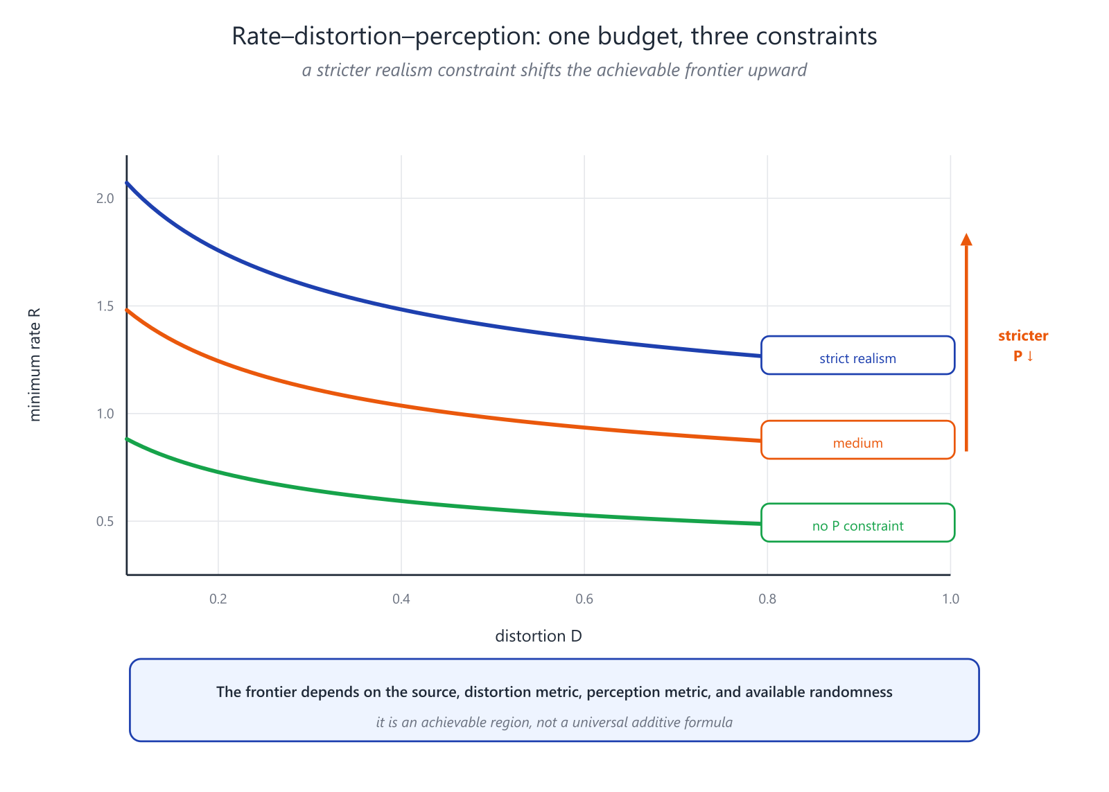
There is no universal additive formula that applies to every source and every metric. The frontier depends on the source, the distortion measure, the distribution discrepancy, available randomness, and the operational coding model.
What a generative decoder buys
An MSE decoder in an ambiguous setting tends toward a posterior mean. A generative decoder can choose one plausible realization from a conditional distribution. The texture may look more convincing, while specific details may differ from the source.
HiFiC demonstrated a practical version of this tradeoff by combining rate, distortion, perceptual, and adversarial terms and evaluating reconstructions both numerically and in a user study. (Mentzer et al., 2020)
The right conclusion is not that a generative codec is “better in general.” It implements a different product contract. If invented details are dangerous, realism cannot replace fidelity. If visual plausibility at extremely low rate is the priority, strict pixel accuracy may be a poor use of the budget.
14.4. Diffusion models: Gaussian noising, denoising, and I–MMSE
Diffusion may look far removed from source coding. Its forward process, however, is a family of Gaussian channels at different signal-to-noise ratios.
Let
Dividing by yields
Each noise level is the same underlying signal observed at a different SNR.
What MSE actually learns
If a network predicts the clean image by minimizing
then the population optimum is the conditional mean:
If it predicts noise through
the optimum is
This is not a diffusion-specific miracle. The conditional mean is the ordinary optimal predictor under squared error. The power of diffusion comes from solving such problems over a continuum or ladder of noise levels.
From a denoiser to the score
For Gaussian corruption,
Given and , the posterior mean, optimal noise predictor, and score are equivalent parameterizations of the same conditional information.
A single MMSE denoiser is still not a generator. A reverse-time SDE or its associated ODE uses the score field across all noise levels to move a random point from a simple base distribution toward the data distribution. The score determines the reverse dynamics in score-based generative modeling. (Song et al., 2021)
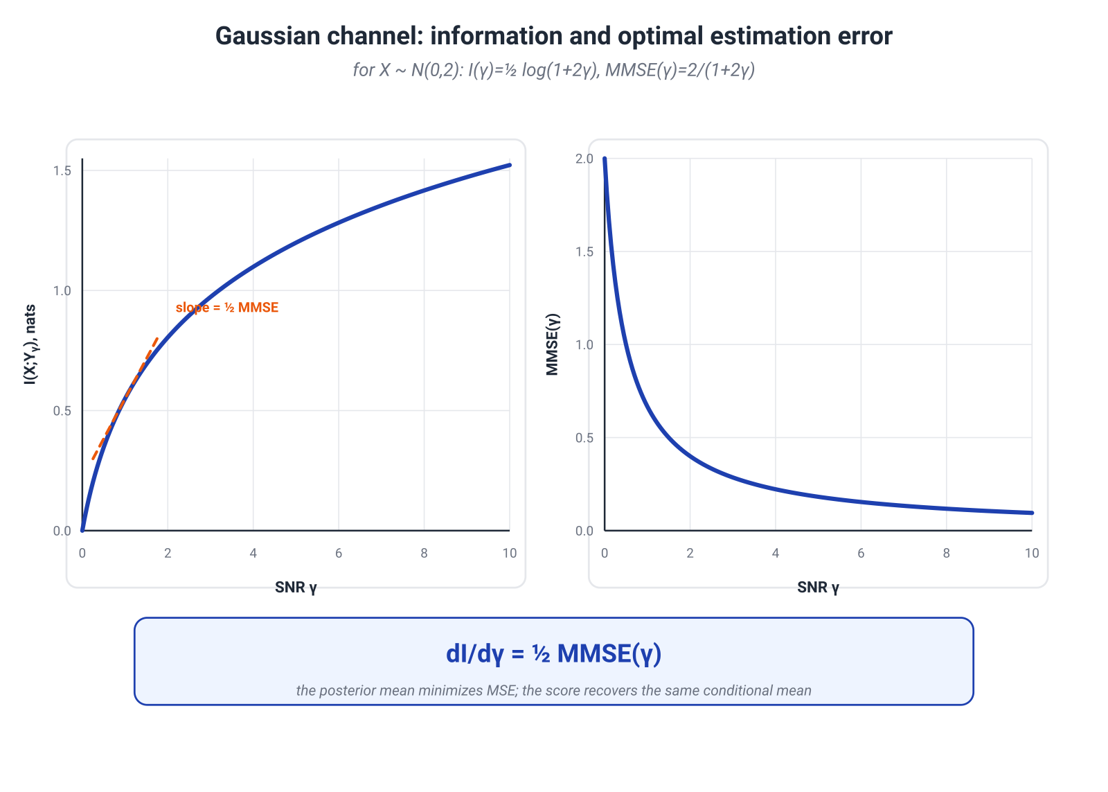
I–MMSE: how much information an increment of SNR buys
For
and mutual information measured in nats,
Here
The identity holds for a broad class of finite-second-moment input distributions. (Guo, Shamai & Verdú, 2005)
The integral form is especially readable:
When the signal remains hard to estimate, a small increase in SNR buys a noticeable amount of information. Once posterior error is already small, additional SNR contributes less.
Where the explanation stops
These identities genuinely connect Gaussian noise, denoising, scores, and mutual information. They do not select:
- the shape of the noise schedule;
- loss weights across noise levels;
- the number of sampling steps;
- the numerical solver;
- a U-Net or Transformer architecture;
- conditioning and guidance mechanisms.
Variational Diffusion Models showed that the continuous-time variational bound can be expressed in SNR terms and, at fixed endpoint SNRs, is invariant in expectation to the detailed schedule shape, although the schedule still affects estimator variance, discretization, and optimization. (Kingma et al., 2021)
This is a representative role for information theory in modern ML: it provides an exact structural skeleton without replacing the entire design problem.
14.5. CLIP and contrastive image–text alignment
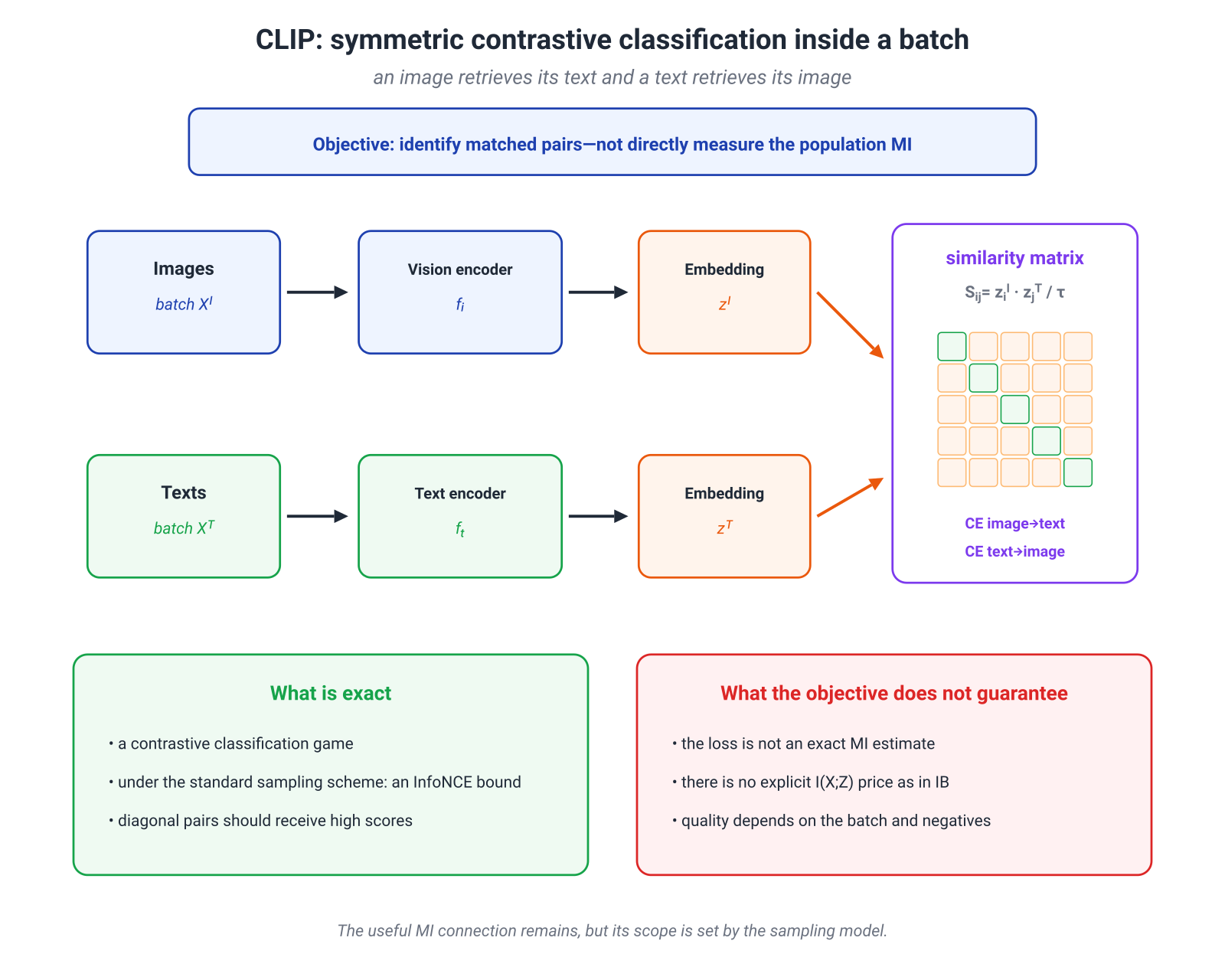
CLIP poses a simple, scalable task: given an image, identify its matching caption among the texts in a batch, and symmetrically identify the matching image for each text.
Let
and let be cosine similarity or an inner product between normalized representations. One half of the symmetric objective is
The visual encoder is therefore trained to distinguish the correct text match among candidates. This is a contrastive classification game, not pixel reconstruction. (Radford et al., 2021)
Connection to InfoNCE
Under the standard sampling scheme—one positive pair from the joint distribution and independent negatives from the marginal—one obtains
This is a substantial connection. Contrastive classification pushes the critic toward a joint-to-product density ratio, and its quality yields a lower bound on mutual information.
The empirical CLIP loss is not, however, an exact numerical measurement of the true MI. The bound depends on the negative-sampling scheme, the critic class, and a population expectation. The quantity caps this particular lower bound, not the information content of the learned representations themselves.
A larger batch supplies more candidates and raises the possible ceiling of the bound. It also changes optimization, the number of false negatives, and computational cost. “More negatives” is an engineering lever, not a monotone law of representation quality.
What training pressure the visual encoder receives
A precise positive statement does not require calling CLIP an IB method:
CLIP amplifies distinctions between images that help identify the associated texts among the available candidates.
This naturally creates strong semantic structure. Objects, actions, styles, and categories that are regularly expressed in captions receive direct training pressure, which helps explain transfer to zero-shot classification and retrieval.
An Information Bottleneck objective would explicitly trade
The standard CLIP loss contains no separate penalty on . It therefore does not imply that the encoder found a minimal sufficient representation or discarded all non-textual information. It is more accurate to speak of task pressure toward relevance than a solved IB problem.
SigLIP illustrates that even within the same broad goal, different training games are possible: it replaces global softmax normalization with a pairwise sigmoid loss. The image–text alignment objective remains, but the statistics of negatives and the computational organization change. (Zhai et al., 2023)
Why the information lens is not the whole explanation
Failures on OCR, counting, or spatial grounding cannot be reduced to one bottleneck. They may also reflect:
- input resolution and patch size;
- the composition of image–text data;
- caption quality;
- the visual encoder architecture;
- the connector between the visual encoder and an LLM;
- post-training and evaluation protocols.
Sufficiency is always relative to a specific target variable. The condition
must be assessed separately for retrieval, OCR, segmentation, and localization. A “semantic embedding” is not a universal sufficient statistic for every visual task.
14.6. Self-supervised visual representations: invariances and collapse prevention
Self-supervised learning replaces human labels with a deliberately constructed prediction problem. A common setup draws two augmented views of the same image:
Augmentations are not merely a way to enlarge the dataset. They are part of the task specification:
If two views are declared equivalent, the model is trained not to rely on their differences.
Color jitter, cropping, blur, and geometric transformations therefore define intended invariances.
There is also an exact boundary. If an augmentation destroys information about a future target , no encoder can recreate it from nothing:
so by data processing,
A strong augmentation can help one downstream task and hurt another. Invariance is always relative to what the representation will later be asked to preserve.
Contrastive methods: SimCLR and MoCo
SimCLR brings two views of the same image together and pushes different images apart using an InfoNCE-like loss. The original study found the augmentation composition, projection head, and sufficient numbers of negatives to be central components. (Chen et al., 2020)
MoCo addresses the same broad problem through a dynamic dictionary: a queue of negative keys and a momentum-updated encoder maintain a large, comparatively consistent candidate set without placing all negatives in the current minibatch. (He et al., 2020)
The MI lower-bound view explains part of the mechanism. The alignment-and-uniformity view explains another: positive pairs should align, while the representation distribution should not collapse to one location.
Self-distillation: BYOL and DINO
If the objective only requires two views to have equal representations, a constant vector is a perfect but useless solution. This is collapse: the matching objective is satisfied, but no useful structure remains.
BYOL avoids conventional negative pairs. An online network predicts a slowly updated target-network representation, while stop-gradient and branch asymmetry alter the optimization dynamics. (Grill et al., 2020)
DINO uses student–teacher self-distillation, centering, sharpening, and multi-crop training. In the original work, self-supervised ViT features exhibited notable spatial structure and performed strongly under k-NN and linear evaluation protocols. (Caron et al., 2021)
These methods can be studied through information-theoretic lenses, but their losses are not standard MI estimators.
Variance and redundancy constraints
VICReg combines:
- an invariance term matching two views;
- a lower bound on per-coordinate variance;
- a covariance penalty across coordinates.
The variance term prevents all samples from becoming one point; the covariance term reduces linear redundancy. (Bardes, Ponce & LeCun, 2021)
Barlow Twins pushes the cross-correlation matrix between two views toward the identity. (Zbontar et al., 2021)
Positive variance does not by itself guarantee semantic usefulness, and zero covariance does not imply independence in general. These terms solve a concrete representation-geometry problem, not the entire question of sufficiency.
Masked modeling: MAE
MAE masks a large fraction of image patches, encodes only the visible ones, and trains a lightweight decoder to reconstruct the missing pixels. (He et al., 2022)
Here, the nontrivial signal comes from predicting hidden content. This is a reconstruction objective, not contrastive classification and not an ordinary InfoNCE bound.
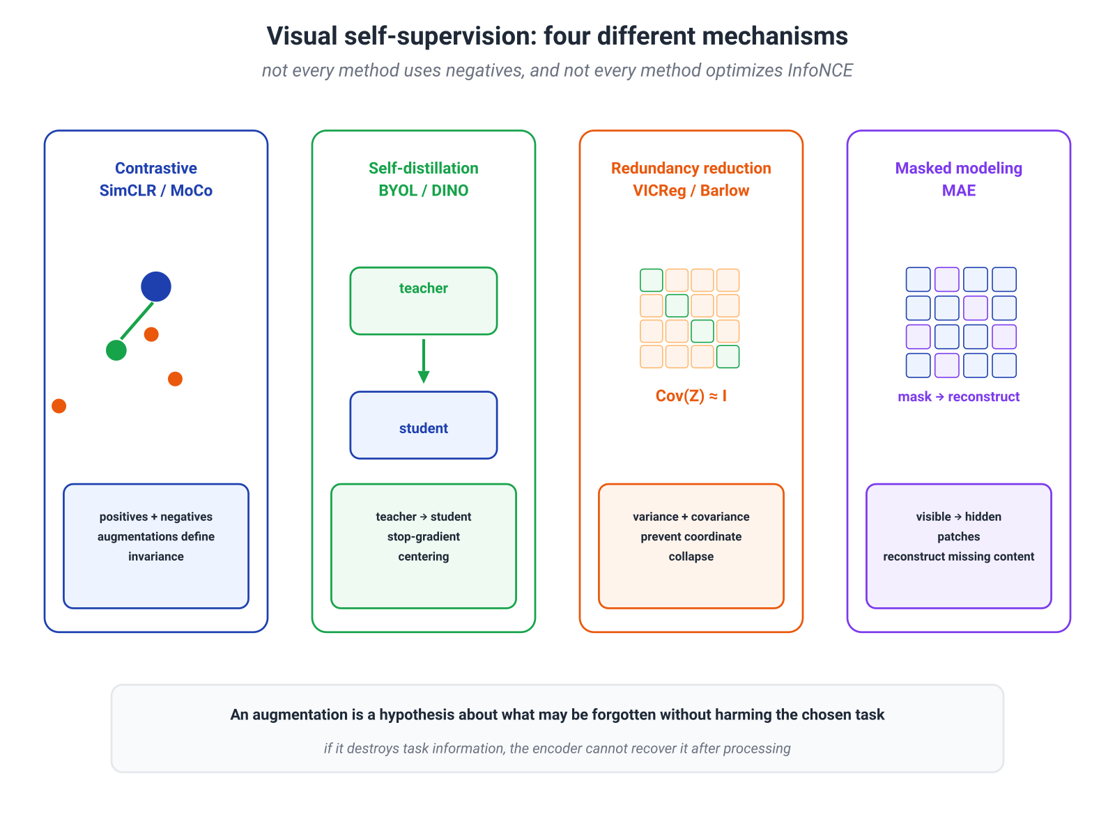
The resulting map is useful:
| Family | What links the two views | How trivial solutions are avoided | What strongly shapes quality |
|---|---|---|---|
| SimCLR, MoCo | contrastive discrimination | negative candidates | augmentations and negative dictionary |
| BYOL, DINO | student–teacher prediction | asymmetry, stop-gradient, teacher dynamics | architecture and update dynamics |
| VICReg, Barlow Twins | statistical matching | variance and decorrelation | chosen batch statistics |
| MAE | masked reconstruction | hidden input content | mask ratio and decoder |
The unifying lesson is not that all these methods “maximize MI.” They construct different ways to preserve predictable structure, impose useful invariances, and prevent collapse. Those differences determine downstream transfer.
14.7. Compressing a CV model: quantization, pruning, and distillation
So far we have compressed an image or a representation. Now the constrained object is the system itself: its serialized size, memory traffic, latency, and energy.
Quantization
For a uniform affine quantizer,
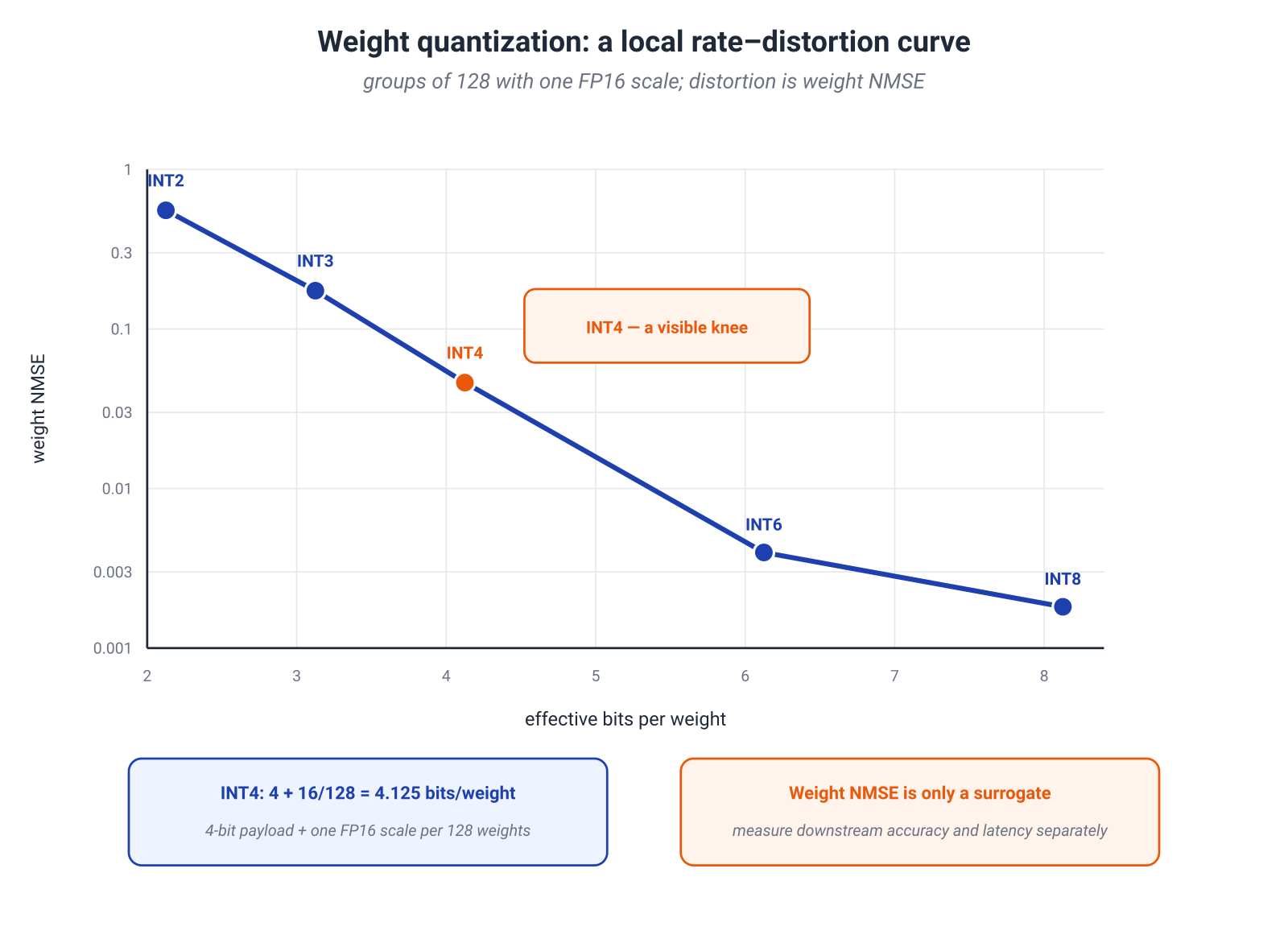
Nominal INT4 means that the code for one quantized value uses four bits. A serialized model also stores scales, zero points, grouping metadata, alignment, and sometimes codebooks.
For example, group-wise INT4 with groups of weights and one 16-bit scale per group uses, before alignment,
bits per original weight.
To turn quantization into a genuine rate–distortion problem, one must choose distortion. The local weight error
is a convenient surrogate, but the same perturbation in different weights may affect activations, logits, and task metrics very differently. Practical methods therefore use calibration data, layer-output reconstruction, Hessian sensitivity, or an end-to-end loss.
PTQ, QAT, and Vision Transformer specifics
Post-training quantization calibrates an already trained network. Quantization-aware training inserts quantization simulation into training so that the parameters can adapt.
Vision Transformers create distinct regimes: LayerNorm inputs, GELU outputs, and attention probabilities have different scales and distribution shapes. FQ-ViT and PTQ4ViT introduced quantizers and calibration criteria tailored to these components. (Lin et al., 2021; Yuan et al., 2021)
Mixed precision as budget allocation
If layer receives bits, an engineering problem takes the form
subject to
This genuinely resembles bit allocation in classical rate–distortion theory. The function , however, belongs to a specific model, dataset, and task. There is no universal closed-form allocation for an arbitrary network.
Pruning: zeros still need a format
Unstructured pruning reduces the number of nonzero parameters, but index and irregular-storage costs remain. At moderate sparsity, a sparse representation may occupy no less space than a dense low-bit tensor and may run poorly on ordinary hardware.
Structured pruning removes channels, heads, or blocks. It is more likely to produce real speedups because it preserves regular operations.
MDL supplies a useful discipline: both values and the sparsity pattern must be paid for. The word “sparse” alone does not determine file size or latency.
Distillation: compressing a function
Knowledge distillation trains a student to approximate a teacher distribution, for example through
It is natural to read this as functional compression: a smaller model receives a tighter computational budget and is asked to reproduce the larger model’s behavior.
Here rate may mean parameters, file size, FLOPs, or latency. Distortion may be output KL, logit error, or degradation in a downstream metric. Until these are stated, “distillation is rate–distortion” remains only a broad analogy.
The synthetic curve below uses groups of 128 weights, p99.9 clipping inside each group, and one stored FP16 scale per group. Its rate and normalized weight MSE therefore describe the same quantization scheme.
A useful deployment report should include:
- serialized model size;
- peak memory;
- target-device latency;
- throughput or energy when measured;
- the end-task metric;
- calibration and robustness after compression.
Nominal bit width is the beginning of the measurement, not its conclusion.
14.8. One CV pipeline, four different information budgets
Consider a text-to-image retrieval system running on an edge device.
- A camera acquires image .
- A codec stores or transmits it when needed.
- A visual encoder produces embedding .
- A text encoder produces query embedding .
- An index searches for nearby vectors.
- A quantized model must fit the device’s memory and latency budget.
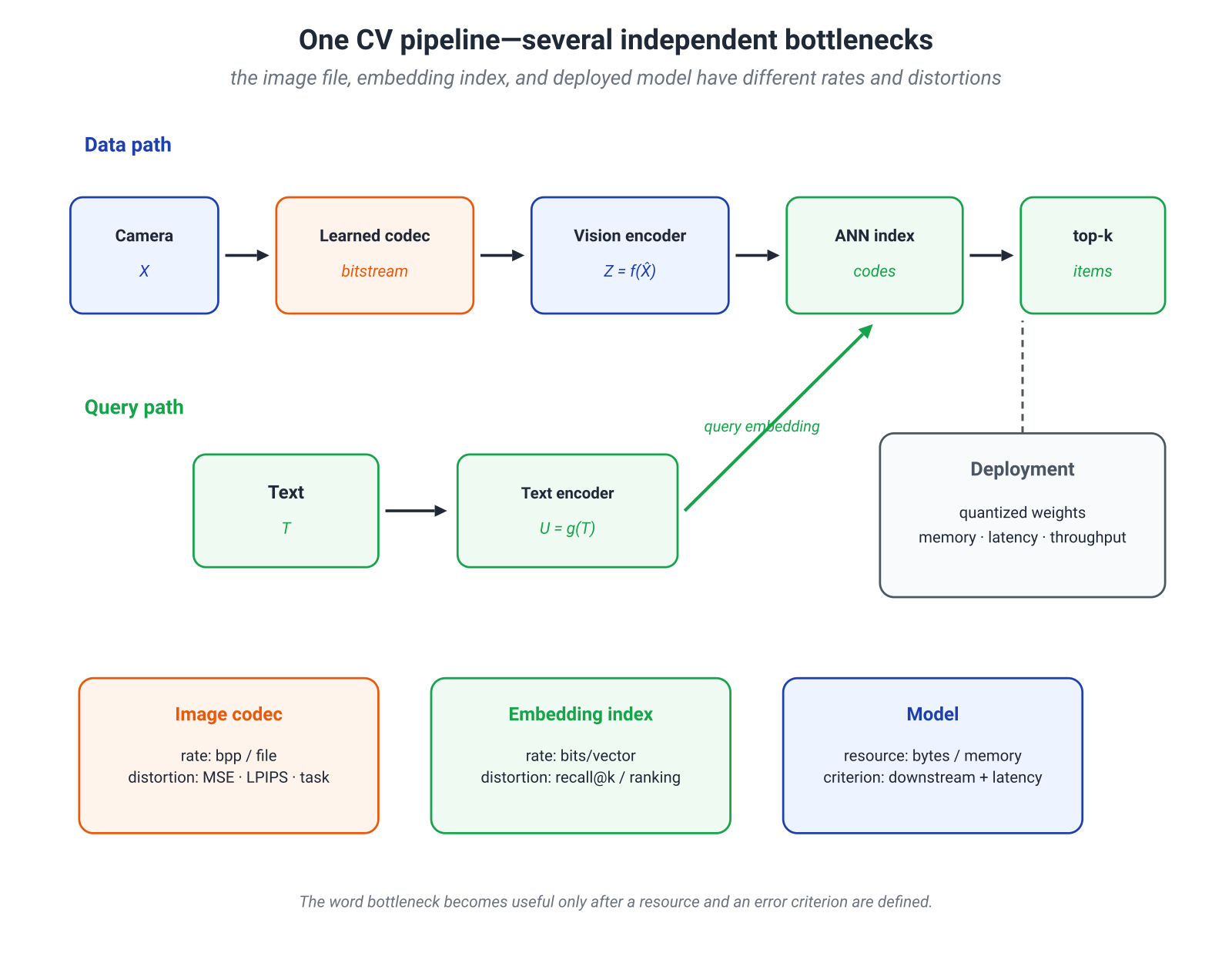
A single product contains several independent bills.
| Component | Rate or resource | Distortion or criterion |
|---|---|---|
| image codec | bits per pixel, file size | MSE, LPIPS, downstream performance |
| visual representation | dimension and statistics of | preservation of task-relevant information |
| retrieval index | bytes per item | recall@K, ranking changes |
| model | bytes, memory, FLOPs, latency | NLL, accuracy, retrieval quality |
Data codec
For a learned codec,
The rate has an operational interpretation.
Representation
Embedding should preserve what matters for text retrieval. Pixel segmentation, precise localization, or image-quality assessment may require a different representation.
One vector cannot be both minimal and sufficient for every possible task. Minimality is always relative to a chosen relevant variable.
Index
Product quantization or binary hashing compresses embeddings. Here rate is bytes per item. Candidate distortions include:
- vector reconstruction error;
- loss of recall@K;
- changes in nearest-neighbor ranking.
These are distinct objectives, and improving one need not improve the others.
Model
INT8 or INT4 reduces model size and memory traffic. Distortion should be measured end to end through retrieval quality, latency, and robustness on the target device.
Diagnostic questions
This pipeline contains several geometries and several random variables that are easy to conflate.
- Cosine distance between embeddings is not an f-divergence between distributions.
- Low coordinate entropy does not guarantee good retrieval.
- Large does not guarantee text relevance.
- Good FID does not guarantee preservation of a particular source detail.
- INT4 does not determine the physical file size without a packing format.
The module therefore reduces to three diagnostic questions:
14.9. Mathematical deepening: two exact calculations
Optional on a first pass. We now make two useful engineering intuitions exact.
14.9.1. When a hyperprior actually saves bits
Let be the true distribution of the main quantized latent and let be a factorized entropy model. Its expected ideal code length is
Introduce an auxiliary variable and a hierarchical model
Its expected bill is
Therefore,
The hyperprior wins when the reduction in model mismatch exceeds the price of side information plus the remaining mismatch of the hierarchical model.
If is a deterministic function of the coded , then : the ideal joint entropy has not increased. A real codec still pays cross-entropy mismatch, finite-precision costs, and headers. If carries additional randomness relative to , its conditional entropy is a genuine cost.
That is the whole mechanism. A hyperprior does not violate Shannon’s limit; it lets a restricted probabilistic model approach the limit more closely.
14.9.2. Gaussian denoising identities
Let
Then
and the posterior variance is
Hence
Now consider
The marginal distribution is
so
The posterior mean is
Substitution yields
In the Gaussian case, the entire bridge between denoising, score estimation, and I–MMSE is visible in closed form. For non-Gaussian data the same structural identities remain, but the posterior mean and score become nonlinear—the quantities a neural network must approximate.
14.11. Conclusion
Computer vision is a useful domain because several meanings of “information” appear in one system and reveal their differences quickly.
In a learned codec, latent probabilities become an actual bitstream. This is an operational connection.
In diffusion, a Gaussian channel links posterior means, scores, and mutual information. This is an exact mathematical mechanism, but not a complete recipe for the generative system.
In CLIP and self-supervised learning, the training objective determines which visual distinctions should become accessible in the representation. Information theory helps interpret that objective, while augmentations, data, embedding geometry, and downstream evaluation still shape the result.
In quantization and pruning, the compressed object is the model itself. Rate must then be measured in the actual format and on the target hardware, while distortion must be measured through system behavior rather than only local weight error.
The main lesson can be stated without metaphor:
Information theory is most useful in computer vision not when every method is renamed a channel or bottleneck, but when it forces us to state exactly what is transmitted, what is reconstructed, and how error is paid.
Primary references
- J. Ballé, V. Laparra, E. P. Simoncelli, End-to-end Optimized Image Compression, 2017.
- J. Ballé et al., Variational Image Compression with a Scale Hyperprior, 2018.
- D. Minnen, J. Ballé, G. Toderici, Joint Autoregressive and Hierarchical Priors for Learned Image Compression, 2018.
- Y. Blau, T. Michaeli, The Perception-Distortion Tradeoff, 2018.
- Y. Blau, T. Michaeli, Rethinking Lossy Compression: The Rate-Distortion-Perception Tradeoff, 2019.
- R. Zhang et al., The Unreasonable Effectiveness of Deep Features as a Perceptual Metric, 2018.
- F. Mentzer et al., High-Fidelity Generative Image Compression, 2020.
- D. Guo, S. Shamai, S. Verdú, Mutual Information and Minimum Mean-Square Error in Gaussian Channels, 2005.
- Y. Song et al., Score-Based Generative Modeling through Stochastic Differential Equations, 2021.
- D. P. Kingma et al., Variational Diffusion Models, 2021.
- A. Radford et al., Learning Transferable Visual Models From Natural Language Supervision, 2021.
- X. Zhai et al., Sigmoid Loss for Language Image Pre-Training, 2023.
- T. Chen et al., A Simple Framework for Contrastive Learning of Visual Representations, 2020.
- K. He et al., Momentum Contrast for Unsupervised Visual Representation Learning, 2020.
- J.-B. Grill et al., Bootstrap Your Own Latent, 2020.
- M. Caron et al., Emerging Properties in Self-Supervised Vision Transformers, 2021.
- A. Bardes, J. Ponce, Y. LeCun, VICReg, 2021.
- J. Zbontar et al., Barlow Twins, 2021.
- K. He et al., Masked Autoencoders Are Scalable Vision Learners, 2022.
- Y. Lin et al., FQ-ViT, 2021.
- Z. Yuan et al., PTQ4ViT, 2021.
- M. Heusel et al., GANs Trained by a Two Time-Scale Update Rule Converge to a Local Nash Equilibrium, 2017.