Module 5. Mutual information: how much one object tells us about another
How to read this module. The main route is §§5.1–5.12. We begin with a familiar ML question about probabilistic prediction, then move to conditional mutual information, representations, noisy labels, InfoNCE, and MI estimation from finite samples. The strong data-processing inequality in §5.5 and Fano's inequality in the exercises are second-pass mathematical deepening.
5.1. A feature is useful only relative to a target
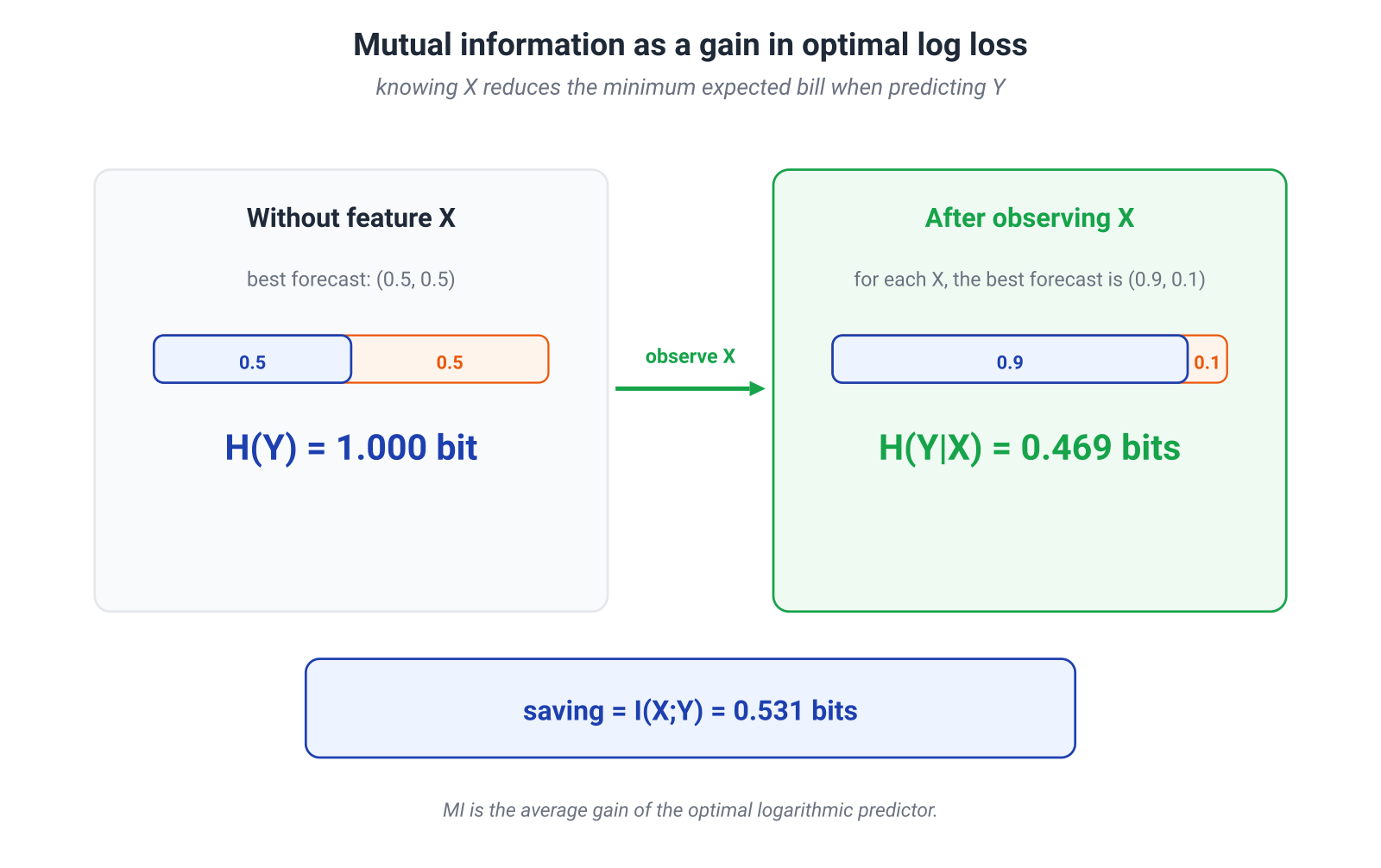
Let the target be a fair bit. Before the model sees any features, its best probabilistic prediction is
The expected logarithmic loss of that prediction is one bit:
Now introduce a feature that agrees with with probability and is flipped with probability . The optimal predictor no longer needs to answer : after observing , it assigns probability to the matching value of . Its expected loss becomes
bits. The feature saves
bits of log loss per observation.
That saving is mutual information:
Mutual information is the expected reduction in optimal logarithmic loss obtained by observing one variable when predicting another.
This interpretation connects classical information theory directly to ML. Mutual information does not answer the vague question “is this a good feature in general?” It answers a precise one:
how much does the feature reduce the irreducible uncertainty of the target under ideal probabilistic prediction on the chosen distribution?
The word ideal matters. A finite model may fail to extract all available information; a finite sample may not support a reliable estimate; the deployment distribution may differ from the training distribution. MI describes a relationship between random variables at the population level, not automatically the performance of a particular trained classifier.
The question appears throughout ML:
- how useful is a feature for a target;
- what does a new feature add beyond those already selected;
- how much target-relevant information did an encoder retain;
- are an image and a caption more strongly matched than a random pair;
- did the target leak into the feature pipeline;
- what common content is retained by two augmentations of the same object?
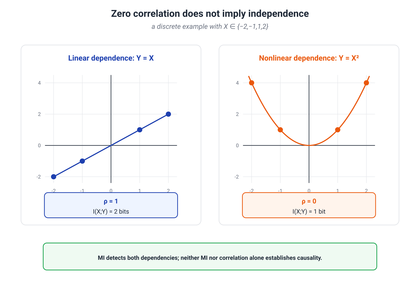
Correlation is a natural first candidate, but it primarily detects linear association. Consider
By symmetry, . Yet is fully determined by and takes two equiprobable values, so
Zero correlation here means no linear trend, not no dependence.
Unless stated otherwise, discrete examples use base-2 logarithms and are measured in bits. ML losses usually use natural logarithms; the corresponding unit is the nat.
5.2. One quantity, three readings
Mutual information has several equivalent forms. Each answers a different question, so it is more useful to move fluently among them than to select a single “primary” definition.
Gain in prediction
Suppose we predict a discrete under log loss. Without access to , the population-optimal forecast is the marginal distribution , and the minimum expected loss is
With access to , the optimal forecast is , and the average minimum loss is
Therefore
The same identity can be read in the opposite direction:
This is why MI is symmetric. Predicting from and predicting from are different tasks, yet the average reduction in logarithmic uncertainty is the same.
Distance from the independent world
The most general formulation is through KL divergence:
is the joint distribution obtained by breaking the dependence while keeping both marginals unchanged. MI therefore measures the average cost of replacing the real joint world by an independent model.
For discrete variables,
The basic properties of KL immediately give
and
This is a fundamental distinction from correlation: zero MI means full statistical independence, not merely the disappearance of one moment.
Overlap of uncertainty
By the chain rule,
For discrete variables this implies
If is a deterministic discrete function, then
This need not equal : a non-invertible map may erase distinctions among values of . A bijection preserves all entropy:
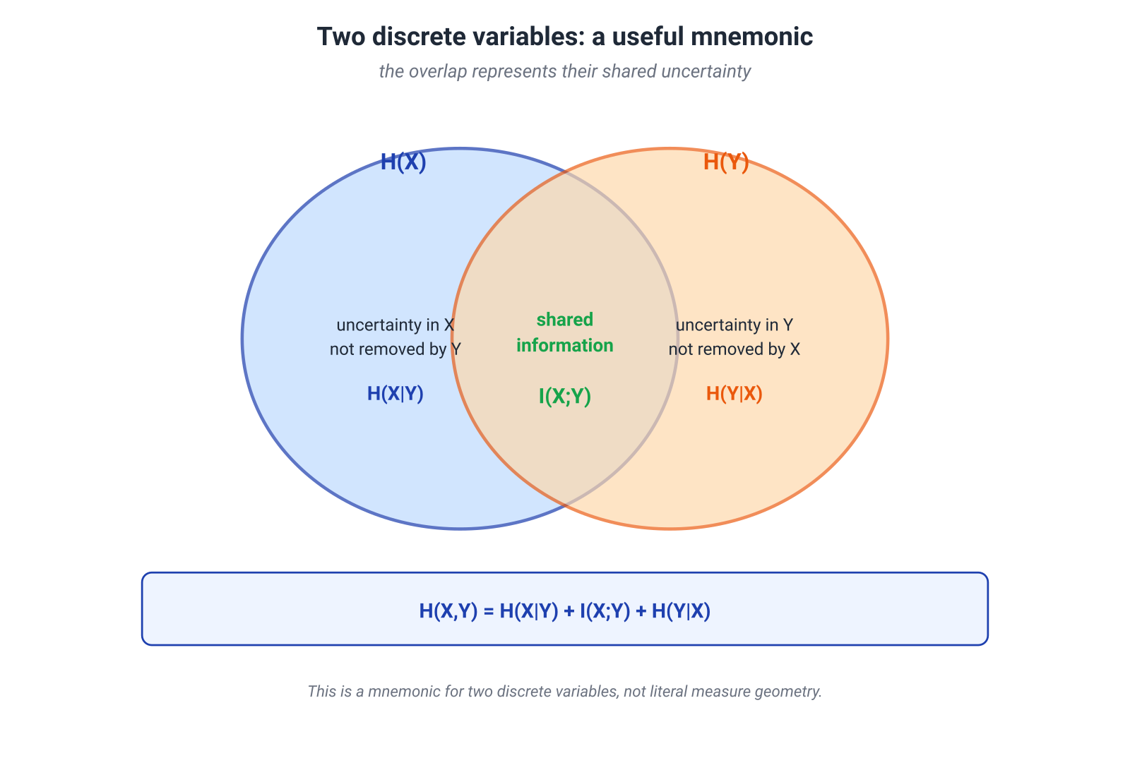
The overlapping-area diagram is a useful mnemonic for two discrete variables, but it is not literal Euclidean geometry. With three or more variables, redundancy, synergy, and interaction information appear; simple circles quickly stop being a reliable map.
Where the safe formulas end. The KL definition remains fundamental for continuous variables. Expressions written as differences of differential entropies require the relevant quantities to be well defined and must avoid indeterminate forms such as . For a continuous non-atomic variable, is typically infinite. Also, self-information normally means the surprisal of an individual outcome, , not the entropy of the distribution.
5.3. PMI: the local log ratio of association
MI averages dependence over all pairs. For a specific pair of outcomes, we use pointwise mutual information (PMI):
It is the logarithm of the factor by which observing changes the probability of relative to its baseline frequency.
For example, let
Under independence the joint probability would be . The actual pair occurs five times more often, so
The sign has a direct interpretation:
- : the pair occurs more often than independence predicts;
- : this particular pair agrees with the independent model;
- : the pair occurs less often than independence predicts.
Unlike MI, an individual PMI value can be negative. Mutual information is its expectation under the true joint distribution:
In NLP, PMI and its variants are used to measure word-context association. The same formula creates a familiar engineering trap: a pair observed once or twice may receive a huge score because the denominator is tiny. Frequency thresholds, smoothing, permutation baselines, or other stability checks are therefore essential. A large logarithm is not yet strong evidence.
5.4. Conditional MI: what a new feature adds beyond known features
Marginal asks whether is useful on its own. In a model with many features, that is not enough. We need to know whether adds anything after another variable is already known.
Define conditional mutual information by
For discrete variables,
This is the expected reduction in optimal log loss obtained by adding to an already available .
The chain rule is
In feature selection, this identity explains two opposing effects.
Redundancy
A new feature may have large but almost zero
because it repeats information already present in the selected set. Temperature in Celsius and Fahrenheit may each be equally informative about a weather label, while the second adds almost nothing after the first.
Synergy
Information may appear only in combination. Let be independent fair bits and
Then
but
Moreover,
Before is known, the first bit is useless; after is known, it determines the label. This is a clean model of interactions that trees, neural networks, and feature crosses may exploit while a univariate filter based on cannot.
Conditional MI provides the right language for incremental value, but not a free algorithm. In high dimensions it is even harder to estimate than marginal MI. Practical methods therefore use approximations, greedy criteria, or direct held-out evaluation of the target metric.
5.5. DPI: an encoder can repackage information, but it cannot print new target bits
Let
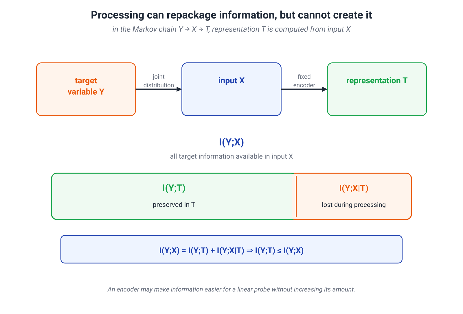
be a Markov chain: the representation is constructed from the input and receives no other path to the target . Then
This is the Data Processing Inequality (DPI).
A fixed transformation can preserve, discard, or repackage target information, but it cannot create information that was absent from the input.
The short proof exposes the source of the loss. By the chain rule,
and also
Markovity gives , hence
The remainder
has a concrete meaning: it is target information that was present in but is no longer available after passing to .
Why classification may become easier after an encoder
At first sight DPI seems to conflict with deep-learning practice: a good encoder can dramatically improve a linear probe. There is no contradiction. DPI limits population information, not its accessibility to a restricted model class.
An encoder can
- make target-relevant information linearly accessible;
- remove nuisance factors that hurt finite-sample learning;
- build useful invariances;
- improve the conditioning and geometry of the problem;
- import inductive bias learned during pretraining.
The information may already have been present in the input but encoded in a form that a simple readout could not exploit. A network need not increase to improve the accuracy of a restricted readout.
Where trained weights enter the probability model
DPI applies to a fixed channel . A pretrained model carries information from its training set in its parameters. If parameters are random, the correct diagram should include them, for example
Once the weights are fixed for a new example, the usual DPI applies under the selected joint distribution. Thus “the network knows nothing beyond the current input” is too crude: it does not create information from nothing, but it can use knowledge encoded in its parameters.
A task-sufficient representation
If and
then retains all information about that was available in :
Such a representation is sufficient for the task. It may discard background color, camera identity, or exact texture when those details do not help predict the target.
Two objectives must be kept separate:
- keep close to ;
- when useful, reduce so that the representation does not carry every detail of the input.
This trade-off motivates the Information Bottleneck:
Module 9 will examine when this formulation is useful and why it should not automatically be treated as a description of the training dynamics of every deterministic neural network.
Mathematical deepening: strong DPI
This subsection can be skipped on a first pass.
Ordinary DPI says only that information does not increase. For some noisy channels, one can obtain a quantitative contraction:
A cascade then yields a geometric upper bound. For a binary symmetric channel with crossover probability , the global KL contraction coefficient is
This is a strong statement about a particular stochastic channel. It does not automatically imply that information in every deep deterministic network must decay exponentially, or that a residual connection has contraction coefficient exactly one. Such a transfer first requires a precise choice of random variables, channel, and supremum domain. SDPI is an exact tool, not a universal architectural metaphor.
5.6. MI, correlation, and causality answer different questions
MI and correlation
Pearson correlation measures normalized linear covariance. MI asks whether the entire joint distribution differs from the product of the marginals.
Therefore
whereas
does not guarantee independence.
For a jointly Gaussian pair,
Natural logarithms give nats; base-2 logarithms give bits. This is a formula for the jointly Gaussian family, not a universal conversion from correlation to MI. Outside that family, a single value of does not determine the full dependence.
MI and causality
Large says that the variables are statistically associated. It does not explain why:
- may cause ;
- may cause ;
- both may depend on a common variable ;
- the association may arise through selection bias;
- the feature may leak information from the future or from preprocessing.
A high-MI feature can be an excellent predictor and a poor intervention variable. Mutual information measures dependence; causal effects require an interventional or causal model.
5.7. Noisy labels: when 100% error still carries one bit
Consider a binary symmetric channel (BSC):
where is a fair bit and is the observed label.
With a uniform input, the observed label is also uniform and
Therefore
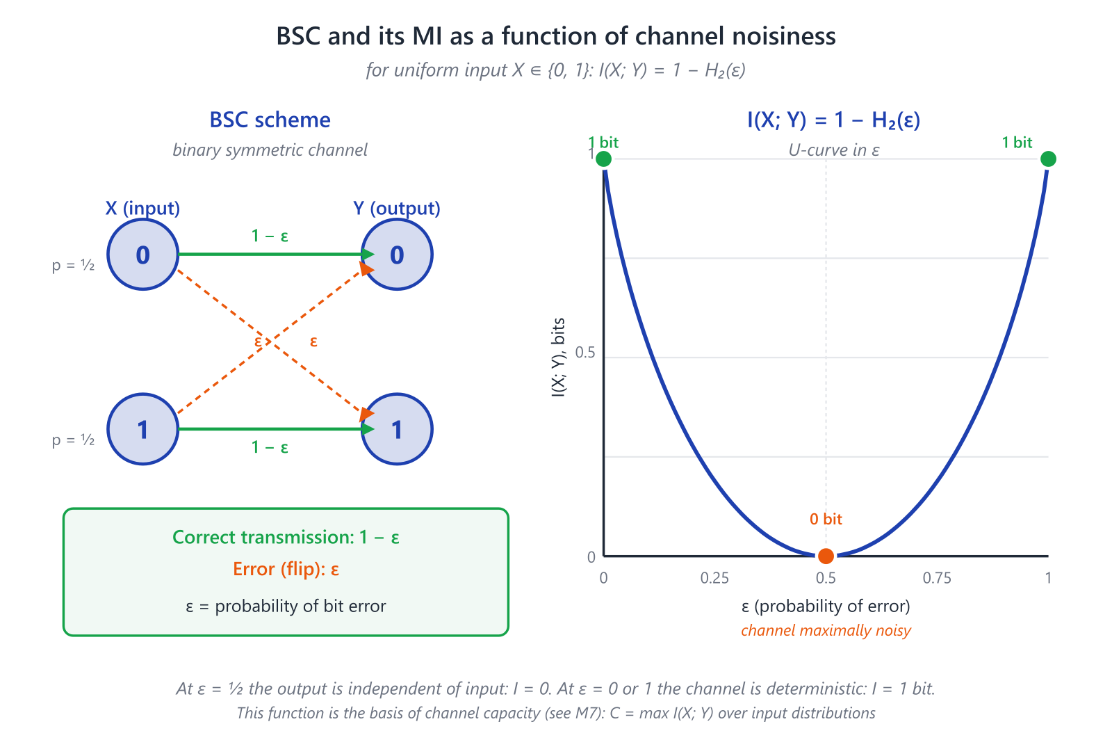
The curve contains three regimes:
- : the label is transmitted perfectly and MI is one bit;
- : the observed label is independent of the true label and MI is zero;
- : the label is always wrong, but the flip is deterministic and invertible, so MI is again one bit.
The last point is especially instructive. Mutual information measures recoverable dependence, not the semantic correctness of a symbol. If an annotator always swaps 0 and 1, the answers are easy to repair once the rule is known. An annotator who flips a fair coin half the time is much worse.
For a BSC, the uniform input achieves capacity:
bits per channel use. In ML this is a clean baseline for symmetric label noise. Real annotation errors often depend on class, example difficulty, annotator, and hidden context; a single is then insufficient.
5.8. Feature selection: a useful filter, not an oracle
The simplest filter ranks features by
Compared with correlation, this is a real extension: nonlinear dependence can be detected. But a universal dependence measure does not make the resulting procedure universally reliable.
| Risk | What happens | What to check |
|---|---|---|
| Redundancy | several features repeat the same information | conditional MI or held-out gain after adding the feature |
| Synergy | features are useless individually but useful jointly | interactions, feature crosses, and an adequate model class |
| Estimation error | the ranking changes with sample size, dimension, and estimator hyperparameters | bootstrap, repeated splits, and a permutation baseline |
| Leakage | validation data influence feature selection | perform selection inside each training fold |
mRMR-style criteria combine relevance with a redundancy penalty. They are useful heuristics, not exact solutions to the general multivariate problem: pairwise penalties need not reveal higher-order synergy.
A practical minimum protocol is:
- define the random variables and the unit of observation;
- treat the estimator and its hyperparameters as part of the training pipeline;
- perform selection only on the training portion of each split;
- compare estimates with a permutation baseline;
- repeat estimation across seeds and sample sizes;
- make the final decision using held-out task performance, not one MI number.
MI is useful here as a filter and diagnostic signal. It does not replace model validation or establish causal usefulness.
5.9. InfoNCE: finding the matched pair among random candidates
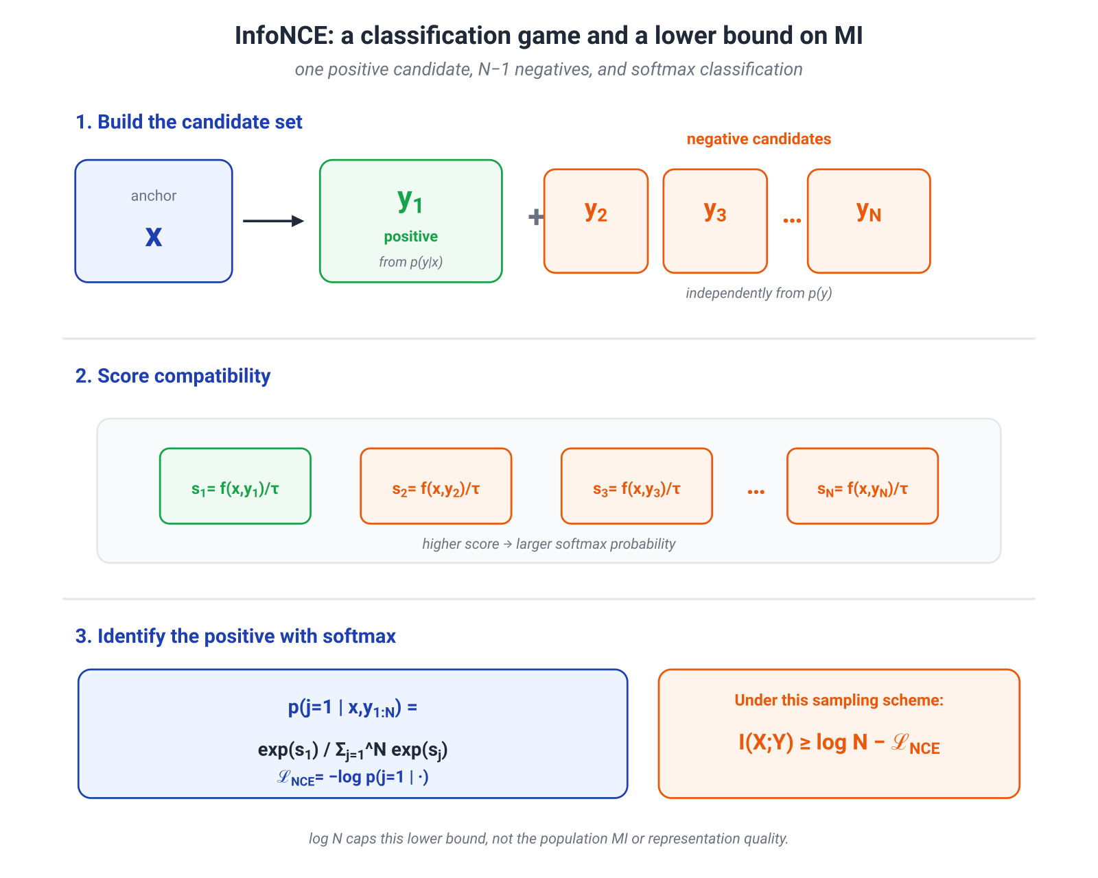
Let be a matched pair: two augmentations of one object, an image and its caption, or an audio segment and its context. For an anchor , draw one positive candidate
and negative candidates
The model receives candidates and must identify the one that forms a genuine pair with . For a compatibility score , the InfoNCE loss is
This is ordinary -class cross-entropy. The classes are unusual: the correct class is the position of the candidate drawn from the conditional distribution, while the others come from the marginal.
Under this standard sampling scheme,
The logarithm base must match the loss. Most implementations use natural logarithms, so the bound is measured in nats.
Why classification is connected to MI
The optimal critic has the form
where cancels inside the softmax. Thus the classifier learns a log density ratio:
how much more likely is candidate next to this than under the dataset-wide baseline?
This is the same local quantity that appeared in PMI. Contrastive classification learns to distinguish the joint distribution from the product of the marginals.
The positive result is strong: reducing the expected InfoNCE loss raises the corresponding lower bound on MI. The exact scope of the result, however, is determined by the candidate-sampling scheme.
Where the exact statement ends
- is a ceiling on this particular lower bound, not on true MI or representation quality;
- the InfoNCE loss is not an exact MI estimate;
- more negative samples do not guarantee better downstream performance;
- in-batch candidates may be dependent and may not match independent draws from ;
- false negatives can push semantically related objects apart;
- temperature, augmentations, batch composition, and critic class change the learning problem.
SimCLR and CLIP use contrastive classification objectives from this family. CLIP symmetrizes the task: each image retrieves its text and each text retrieves its image. The accurate statement is that such objectives are connected to MI through a contrastive bound under an appropriate probabilistic model. Saying that “CLIP literally measures the true MI between images and text” would go beyond the mathematics.
Not all self-supervised learning is InfoNCE. BYOL, SimSiam, and DINO use different mechanisms to avoid collapse and do not reduce to the standard classification of one positive among independent negatives.
5.10. Why MI is hard to estimate from samples
The formula for mutual information is short. Reliable estimation from finite data is not.
Discrete plug-in estimator
For finite alphabets, empirical frequencies can be substituted directly:
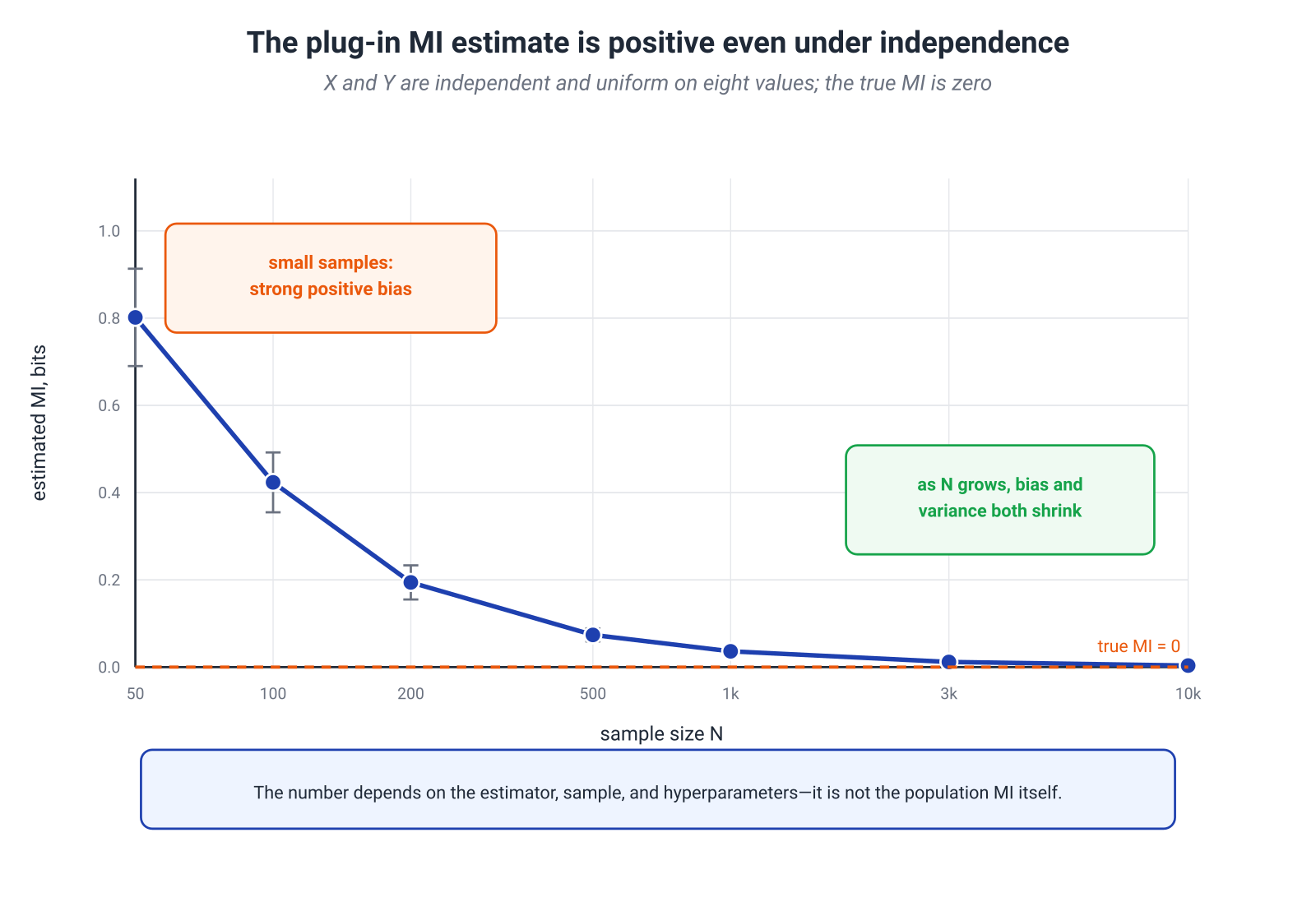
When the contingency table is small and well populated, the method is transparent. With many cells it becomes sparse: accidental single observations look like structure, and zero counts require smoothing.
Binning continuous variables
Binning converts continuous data into discrete data. The result depends on the number and location of bins, outliers, sample size, and dimension. Bins that are too coarse erase dependence; bins that are too fine memorize sampling noise.
Nearest-neighbor estimators
KSG-style methods choose a local scale through distances to the nearest neighbors. In low dimensions they are often more useful than fixed binning, but they remain sensitive to the metric, dimensionality, ties, and preprocessing. The choice of again controls a bias-variance trade-off.
Neural variational bounds
MINE and related methods train a critic for a variational lower bound on
This turns MI into a differentiable objective, but it does not remove the statistical difficulty. The critic can overfit, and both estimates and gradients may have substantial bias or variance. There is a fundamental limitation for lower bounds: without distributional assumptions, a high-confidence lower bound built from observations cannot in general grow reliably much faster than order .
Two statements must therefore be separated:
- a neural network can output an arbitrarily large number;
- that number is a guaranteed lower bound on population MI.
The first is possible. The second requires a theorem, assumptions, and a generalization argument.
A protocol that makes the number meaningful
Before reporting “MI = 3.7 bits,” ask:
- What random variables and population distribution are being defined?
- Are the variables discrete or continuous?
- Which estimator is used, and what assumptions does it make?
- Was the estimator trained and reported on the same data, or is there held-out evaluation?
- What is the permutation baseline?
- Is the result stable across sample sizes, seeds, and estimator hyperparameters?
In representation learning, MI is often more useful as a design principle or comparative diagnostic than as an absolute measuring instrument.
5.11. Attention entropy is not mutual information
After softmax, attention weights form a distribution over keys:
For query , one can therefore compute
This quantity exactly describes concentration of the weights:
- low entropy means that mass is concentrated on a few positions;
- high entropy means that it is spread more broadly.
MI, however, requires a joint distribution of two random variables. A single row of attention weights does not provide that object. Moreover, the layer output depends not only on but also on value vectors, the residual stream, later layers, and nonlinearities.
Attention entropy may therefore be a useful descriptive statistic of routing, but it does not automatically equal
- information transmitted between tokens;
- the causal influence of a position on the answer;
- a complete explanation of the model's decision;
- evidence that sharper or more diffuse attention is better.
There is no need to abandon information-theoretic language. We must first define random variables, a channel, and a joint distribution, and only then compute MI. Module 7 will do this for genuine communication channels; attention will return as a mechanism whose channel interpretation requires an explicit model.
5.12. What to carry into ML practice
Mutual information unifies several problems that ML often discusses in different vocabularies:
- dependence: how far the joint distribution is from an independent model;
- predictive value: how much optimal log loss a feature saves;
- incremental value: what a new feature adds beyond known features;
- representations: how much target-relevant information an encoder preserves;
- contrastive learning: how well a matched pair can be found among random candidates;
- limits of processing: what cannot be recovered after an irreversible transformation.
The central formula should no longer read as an abstract difference of entropies:
It says:
before observing , optimal log loss costs bits; after observing it, the cost is ; the difference is the informational value of for .
For practical work, keep three objects separate:
InfoNCE can be an effective objective without being an accurate MI meter. A large MI estimate can be produced by an overfit critic. A high-MI feature can be leakage. A representation can improve a linear readout without violating DPI or increasing true target information.
These are not exceptions that weaken an elegant theory. They are what mature use of the theory looks like: first identify the exact positive result, then determine which object the code actually computes.
5.14. Sources and further reading
- C. E. Shannon, A Mathematical Theory of Communication, 1948.
- T. M. Cover, J. A. Thomas, Elements of Information Theory, 2nd ed., 2006.
- A. van den Oord, Y. Li, O. Vinyals, Representation Learning with Contrastive Predictive Coding, 2018.
- B. Poole et al., On Variational Bounds of Mutual Information, 2019.
- M. I. Belghazi et al., MINE: Mutual Information Neural Estimation, 2018.
- D. McAllester, K. Stratos, Formal Limitations on the Measurement of Mutual Information, 2020.
- A. Kraskov, H. Stögbauer, P. Grassberger, Estimating Mutual Information, 2004.
- N. Tishby, F. C. Pereira, W. Bialek, The Information Bottleneck Method, 2000.
- Y. Polyanskiy, Y. Wu, Strong Data-Processing Inequalities for Channels and Bayesian Networks, 2017.
- T. Chen et al., A Simple Framework for Contrastive Learning of Visual Representations, 2020.
- A. Radford et al., Learning Transferable Visual Models From Natural Language Supervision, 2021.
- M. Caron et al., Emerging Properties in Self-Supervised Vision Transformers, 2021.
- J.-B. Grill et al., Bootstrap Your Own Latent: A New Approach to Self-Supervised Learning, 2020.
- X. Chen, K. He, Exploring Simple Siamese Representation Learning, 2020.
Module 6 turns from dependence to source coding. Entropy will stop being only a measure of uncertainty and become an operational limit on average code length.