Module 4. Jensen's inequality: when averaging meets nonlinearity

How to read this module. Sections 4.1–4.5 form the main route. A single theorem will run through three familiar ML constructions: ensembles, the ELBO, and the contraction of KL under coarse-graining. The mathematical deepening on the Jensen gap and Bregman divergence can wait for a second pass. To move on to Module 5, it is enough to understand the direction of the inequality, its equality conditions, and two working consequences: ensemble guarantees and the log-sum inequality.

4.1. Average first, or evaluate the loss first?

In machine learning, an average rarely appears alone. It is usually followed or preceded by a nonlinearity: a logarithm, an exponential, a square, softmax, or logsumexp. Once a nonlinear map enters, the order of operations matters.

Consider the shortest possible example. Two models assign the observed class probabilities

$$q_1(y\mid x)=0.9, \qquad q_2(y\mid x)=0.1.$$

Their average NLL is

$$\frac{-\ln 0.9-\ln 0.1}{2} \approx 1.204\ \text{nats}.$$

If we average the probabilities first, we obtain $0.5$, followed by

$$-\ln 0.5\approx0.693\ \text{nats}.$$

Neither original model has improved. We merely changed the order of two operations:

$$-\log\left(\frac{q_1+q_2}{2}\right) \qquad\text{instead of}\qquad \frac{-\log q_1-\log q_2}{2}.$$

The difference comes from the curvature of $-\log u$. The same pattern reappears in more substantial settings:

• an ensemble mixes predictions before receiving a logarithmic score;
• a latent-variable model sums or integrates over hidden explanations before taking a logarithm;
• a data transformation merges states before we compare the resulting distributions by KL;
• logit averaging passes through the convex logsumexp function.

Each case asks the same question:

$$\phi(\mathbb E X) \qquad\text{or}\qquad \mathbb E[\phi(X)]?$$

Jensen's inequality is a compass for situations in which we try to move an average through a nonlinearity. It tells us the direction of the change; the Jensen gap tells us the price of the swap.

Unless stated otherwise, this module uses natural logarithms. Changing the base only multiplies logarithmic quantities by a positive constant and therefore does not change any inequality direction.

4.2. Jensen's inequality: curvature sets the direction

From a chord to a random variable

Let $C\subseteq\mathbb R^d$ be convex. A function $\phi:C\to\mathbb R$ is convex if, for all $x_1,x_2\in C$ and $\lambda\in[0,1]$,

$$\phi\bigl(\lambda x_1+(1-\lambda)x_2\bigr) \le \lambda\phi(x_1)+(1-\lambda)\phi(x_2).$$

Geometrically, the chord joining two points on the graph lies above the graph. For a concave function, the inequality reverses.

The weighted finite form is

$$\phi\left(\sum_{j=1}^M\lambda_jx_j\right) \le \sum_{j=1}^M\lambda_j\phi(x_j), \qquad \lambda_j\ge0, \quad \sum_j\lambda_j=1.$$

Passing from a finite mixture to a random variable gives Jensen's familiar expectation form. If the required expectations exist and $X$ takes values in $C$, then

$$\boxed{ \phi(\mathbb E[X]) \le \mathbb E[\phi(X)] }.$$

For concave $\phi$,

$$\boxed{ \phi(\mathbb E[X]) \ge \mathbb E[\phi(X)] }.$$

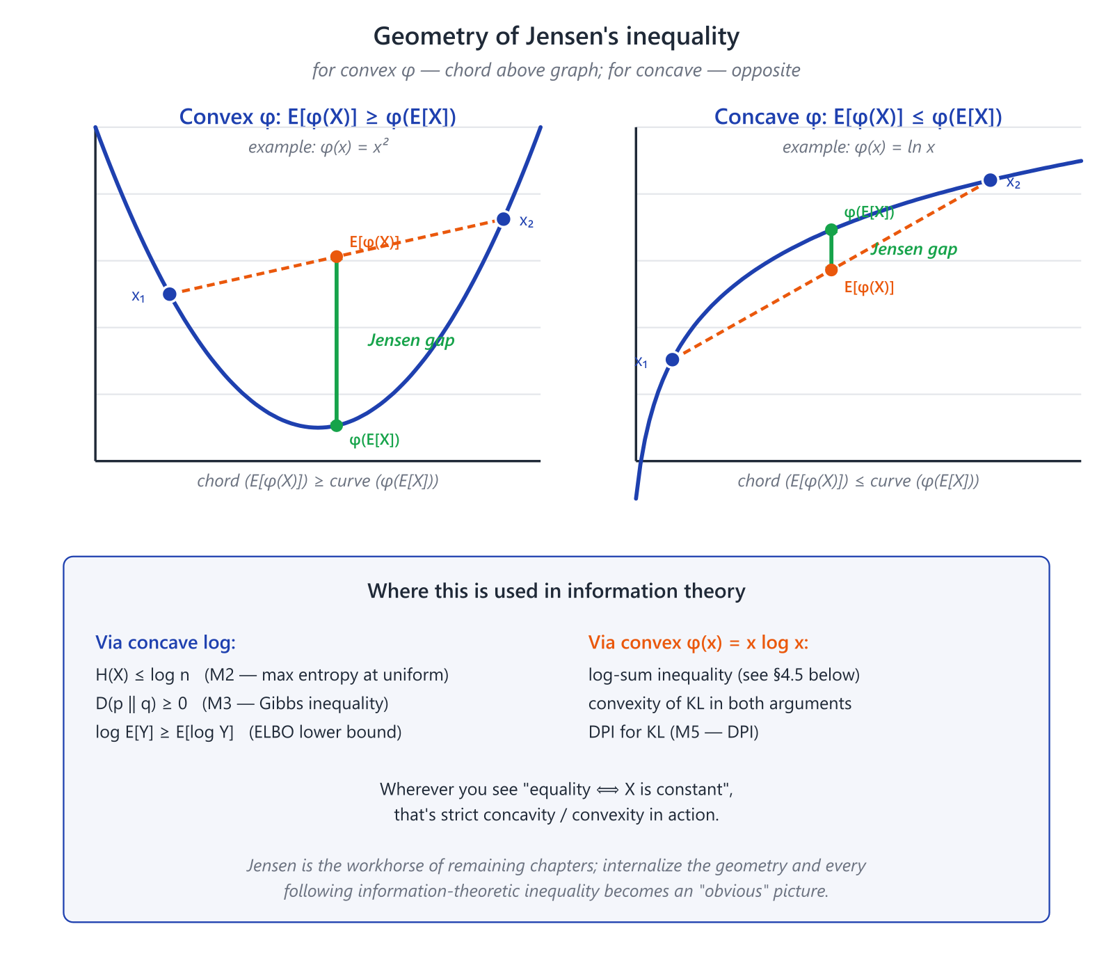
Four functions will keep returning throughout the course:

The square gives the most familiar special case:

$$(\mathbb E X)^2\le\mathbb E[X^2],$$

or, equivalently,

$$\operatorname{Var}(X) = \mathbb E[X^2]-(\mathbb E X)^2 \ge0.$$

A short proof worth seeing once

Assume that $\phi$ is differentiable and convex, and let

$$m=\mathbb E X.$$

A tangent hyperplane to a convex function is a global lower bound:

$$\phi(x) \ge \phi(m)+\nabla\phi(m)^\top(x-m).$$

Take expectations:

$$\begin{aligned} \mathbb E[\phi(X)] &\ge \phi(m)+\nabla\phi(m)^\top(\mathbb E X-m)\\ &=\phi(m). \end{aligned}$$

The linear term vanishes precisely because the tangent is taken at the mean $m$. That is the entire mechanism. In the general nondifferentiable case, a supporting subgradient plays the same role; the differentiable version is enough for the ML applications below.

When does the inequality become an equality?

If $\phi$ is strictly convex on the convex hull of the essential support of $X$, then

$$\phi(\mathbb E X)=\mathbb E\phi(X)$$

is possible only when $X$ is almost surely constant. For a finite mixture with positive weights, all arguments that actually participate in the mixture must coincide.

For a function that is convex but not strictly convex, nontrivial equality cases are possible—for example, when the support lies entirely in a region on which the function is affine.

This is not merely a technical footnote. It answers a practical question: when does averaging actually change anything? If the models provide the same relevant argument, Jensen creates no gain; if their arguments differ and the function bends between them, the gap is nonzero.

Mathematical deepening: the gap, curvature, and Bregman divergence

For convex $\phi$, define the Jensen gap

$$J_\phi(X) := \mathbb E\phi(X)-\phi(\mathbb E X) \ge0.$$

If $X$ is scalar, concentrated near $m=\mathbb E X$, and $\phi$ is twice differentiable, a Taylor expansion gives the local approximation

$$J_\phi(X) \approx \frac12\phi''(m)\operatorname{Var}(X).$$

In several dimensions, the corresponding expression is

$$J_\phi(X) \approx \frac12 \operatorname{tr} \left( \nabla^2\phi(m)\operatorname{Cov}(X) \right).$$

This gives a useful engineering intuition: averaging has an effect only when there is both dispersion in the arguments and curvature in the relevant directions. The slogan “more diverse models always make a better ensemble” is therefore too crude. What matters is diversity in the predictions along directions to which the loss is curved.

For differentiable convex $\phi$, define the Bregman divergence

$$D_\phi(x,m) = \phi(x)-\phi(m)-\nabla\phi(m)^\top(x-m).$$

Once again the linear term disappears after averaging:

$$\boxed{ J_\phi(X) = \mathbb E D_\phi(X,\mathbb E X) }.$$

For $\phi(x)=x^2/2$, the right-hand side is $\operatorname{Var}(X)/2$. Thus the Jensen gap can be read as an average curvature-aware displacement from a random argument to its mean. This connection is useful, but not required for the main route.

4.3. Ensembles: an exact guarantee for log loss

Suppose $M$ models produce distributions

$$q_1(y\mid x),\ldots,q_M(y\mid x),$$

with weights $\lambda_j\ge0$ summing to one. There are at least two natural ways to build an ensemble, and they define different predictive models.

Mixing probabilities

Define the arithmetic mixture

$$q_{\mathrm{mix}}(y\mid x) = \sum_{j=1}^M\lambda_jq_j(y\mid x).$$

For the observed label $y$, the function $-\log u$ is strictly convex, so

$$\boxed{ -\log q_{\mathrm{mix}}(y\mid x) \le \sum_{j=1}^M \lambda_j[-\log q_j(y\mid x)] }.$$

This is stronger than an average test-set statement: it holds for every individual example. Averaging it over a dataset preserves the inequality.

Equality holds when all positively weighted models assign the observed class the same probability. Their full distributions may still differ: per-example NLL only sees the coordinate of the observed class.

The formula compares the mixture with the average member, not with the best member. Nor does it automatically promise higher top-1 accuracy, better calibration under every distribution, or robustness to dataset shift. That is not a weakness of the result; it is its exact scope: for fixed predictions, a probability mixture is no worse than the average member under log loss.

Averaging logits

Let

$$q_j=\operatorname{softmax}(z_j)$$

and average logits rather than probabilities:

$$\bar z = \sum_j\lambda_jz_j.$$

The cross-entropy loss for class $y$ is

$$\ell(z,y) = \operatorname{LSE}(z)-z_y, \qquad \operatorname{LSE}(z)=\log\sum_k e^{z_k}.$$

logsumexp is convex, and subtracting a linear term preserves convexity. Hence

$$\boxed{ \ell(\bar z,y) \le \sum_j\lambda_j\ell(z_j,y) }.$$

This ensemble is also no worse than the average member under NLL. Its distribution, however, is not the arithmetic mixture. From the softmax definition,

$$\operatorname{softmax}(\bar z)_k = \frac{ \prod_j q_j(k)^{\lambda_j} }{ \sum_r\prod_jq_j(r)^{\lambda_j} }.$$

Thus logit averaging produces a normalized geometric mean, also known as a logarithmic opinion pool.

The distinction has a useful qualitative interpretation.

• An arithmetic mixture tolerates disagreement: one member assigning a high probability can keep a class alive.
• A geometric mixture demands more agreement: a very small probability from one member suppresses the class more strongly.

For finite logits, equality in the logit inequality occurs, in particular, when all models define the same softmax distribution—that is, when their logits differ only by additive constants shared across classes.

Neither method wins universally

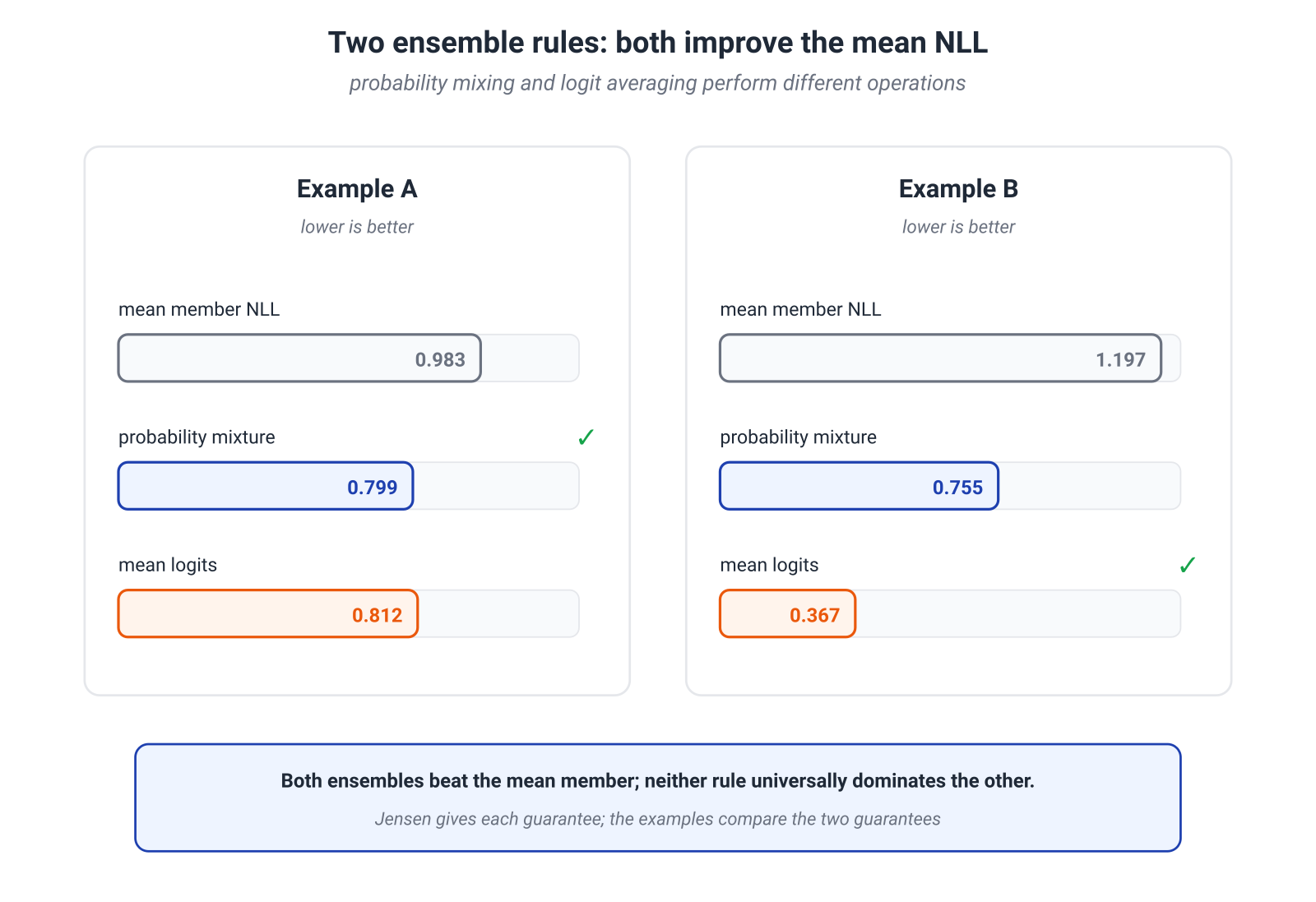
Consider two examples with equal weights and class $1$ observed.

The arithmetic mixture wins in the first example; the geometric mixture wins in the second. Both satisfy their Jensen guarantee, but there is no universal ordering between them.

Implementation detail: these are different lines of code

If the models already return logits, compute the probability mixture stably in log space:

import torch
import torch.nn.functional as F

# logits: [num_models, num_classes]
# weights: [num_models], positive and summing to one
# target: scalar class index
log_probs = F.log_softmax(logits, dim=-1)
log_weights = weights.log()

# Arithmetic mixture of probabilities, computed stably.
log_q_mix = torch.logsumexp(
    log_probs + log_weights[:, None], dim=0
)
loss_probability_mix = -log_q_mix[target]

# Averaging logits gives a normalized geometric pool.
mean_logits = (weights[:, None] * logits).sum(dim=0)
loss_logit_mix = F.cross_entropy(
    mean_logits[None, :],
    torch.tensor([target], device=logits.device),
)

Averaging logits is not a numerically convenient substitute for averaging probabilities. It is a different operation and may produce a substantially different prediction.

4.4. The ELBO: the logarithm sits outside hidden explanations

In a latent-variable model, an observation $x$ can have many hidden explanations $z$. The marginal likelihood adds them up:

$$p_\theta(x) = \int p_\theta(x,z)\,dz.$$

Training requires

$$\log p_\theta(x) = \log\int p_\theta(x,z)\,dz,$$

but the integral is often intractable. The familiar structural problem has returned: the logarithm is applied after summing over hidden states.

Introduce a variational distribution $q_\phi(z\mid x)$ that is positive wherever $p_\theta(x,z)>0$. Then

$$\begin{aligned} \log p_\theta(x) &= \log\int q_\phi(z\mid x) \frac{p_\theta(x,z)}{q_\phi(z\mid x)}\,dz\\ &= \log\mathbb E_{q_\phi(z\mid x)} \left[ \frac{p_\theta(x,Z)}{q_\phi(Z\mid x)} \right]. \end{aligned}$$

The logarithm is concave, so Jensen reverses the inequality:

$$\boxed{ \log p_\theta(x) \ge \mathbb E_{q_\phi(z\mid x)} \left[ \log p_\theta(x,Z)-\log q_\phi(Z\mid x) \right] }.$$

The right-hand side is the evidence lower bound, or ELBO:

$$\operatorname{ELBO}(x) := \mathbb E_{q_\phi(z\mid x)} \left[ \log p_\theta(x,Z)-\log q_\phi(Z\mid x) \right].$$

Here Jensen does more than certify the existence of a bound. It turns a difficult log integral into an expectation that can be estimated with samples from $q_\phi$ and optimized with stochastic gradients.

The gap is known exactly

Using

$$p_\theta(z\mid x) = \frac{p_\theta(x,z)}{p_\theta(x)},$$

we obtain

$$\begin{aligned} \log p_\theta(x)-\operatorname{ELBO}(x) &= \mathbb E_{q_\phi} \left[ \log\frac{q_\phi(Z\mid x)}{p_\theta(Z\mid x)} \right]\\ &= D_{\mathrm{KL}} \bigl( q_\phi(z\mid x) \|p_\theta(z\mid x) \bigr). \end{aligned}$$

Therefore

$$\boxed{ \log p_\theta(x) = \operatorname{ELBO}(x) + D_{\mathrm{KL}} \bigl(q_\phi(z\mid x)\|p_\theta(z\mid x)\bigr) }.$$

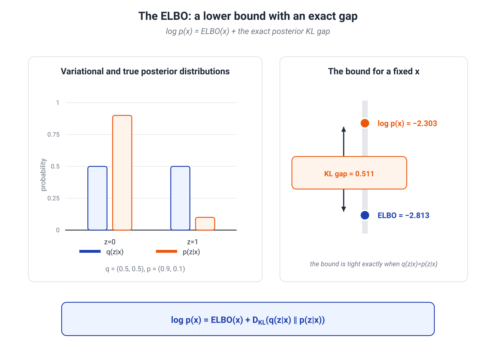
Jensen's equality condition now receives a probabilistic interpretation. The importance weight

$$W(z) = \frac{p_\theta(x,z)}{q_\phi(z\mid x)}$$

must be constant under $z\sim q_\phi$. This happens exactly when

$$q_\phi(z\mid x)=p_\theta(z\mid x)$$

almost everywhere. In that case $W(z)=p_\theta(x)$ and the bound is tight.

A small discrete example

For a fixed $x$, suppose

$$p(x,z=0)=0.09, \qquad p(x,z=1)=0.01.$$

Then

$$p(x)=0.1, \qquad p(z\mid x)=(0.9,0.1).$$

Take the crude approximation

$$q(z\mid x)=(0.5,0.5).$$

We have

$$\log p(x)=\ln0.1\approx-2.303,$$

and

$$\operatorname{ELBO}(x) = \frac12\ln\frac{0.09}{0.5} + \frac12\ln\frac{0.01}{0.5} \approx-2.813.$$

The gap is

$$-2.303-(-2.813) \approx0.511\ \text{nats},$$

which is exactly

$$D_{\mathrm{KL}}\bigl((0.5,0.5)\|(0.9,0.1)\bigr).$$

The value $0.511$ is not a penalty inserted by hand. It is the exact price of using $q$ instead of the true posterior.

The form familiar from VAEs

If the joint model factorizes as

$$p_\theta(x,z)=p(z)p_\theta(x\mid z),$$

then the ELBO becomes

$$\boxed{ \operatorname{ELBO}(x) = \mathbb E_{q_\phi(z\mid x)} [\log p_\theta(x\mid z)] - D_{\mathrm{KL}} \bigl(q_\phi(z\mid x)\|p(z)\bigr) }.$$

The first term is often called the reconstruction term, although mathematically it is an expected conditional log likelihood and its exact form depends on the decoder. The second compares the approximate posterior with the prior. It follows from the probabilistic decomposition; it is not an external regularizer attached to the objective after the fact.

The positive result is already strong:

• maximizing the ELBO raises a computable lower bound on $\log p_\theta(x)$;
• the tightness of the bound is determined by the KL divergence to the true posterior;
• a richer variational family can reduce the best achievable variational gap.

The boundary is equally important. A higher ELBO does not guarantee a global optimum, a useful latent representation for every downstream task, or an easy optimization problem. IWAE, the amortization gap, and posterior collapse belong in Module 9, where the full VAE setting will be available.

4.5. The log-sum inequality: what is lost when states are merged

Suppose $P$ and $Q$ differ over four states, after which we merge those states into two groups. We have discarded detail. Can the KL distinguishability of the distributions increase?

No. The algebraic mechanism behind this fact is the log-sum inequality.

Statement

Let $a_i,b_i\ge0$, with

$$A=\sum_i a_i, \qquad B=\sum_i b_i.$$

Use the conventions

$$0\log\frac0b:=0, \qquad a\log\frac a0:=+\infty\quad(a>0).$$

Then

$$\boxed{ \sum_i a_i\log\frac{a_i}{b_i} \ge A\log\frac AB }.$$

If $A,B>0$ and the left-hand side is finite, equality holds exactly when the normalized vectors agree:

$$\frac{a_i}{A} = \frac{b_i}{B}$$

for all relevant $i$. Equivalently, the ratios $a_i/b_i$ are constant.

Why this is the same nonnegativity of KL

Normalize the sequences:

$$p_i=\frac{a_i}{A}, \qquad q_i=\frac{b_i}{B}.$$

Then

$$\begin{aligned} \sum_i a_i\log\frac{a_i}{b_i} &= A\sum_i p_i \log\frac{Ap_i}{Bq_i}\\ &= A\log\frac AB + A D_{\mathrm{KL}}(P\|Q)\\ &\ge A\log\frac AB. \end{aligned}$$

The log-sum inequality is not a separate trick to memorize next to KL. It is KL nonnegativity after the right normalization.

It can also be derived directly from Jensen's inequality applied to the convex function $u\log u$, with weights $b_i/B$. The two proofs expose the same structure from different sides.

Joint convexity of KL: mixing hides the component index

Let $(P_j,Q_j)$ be pairs of distributions with weights $\lambda_j$. For each outcome, apply log-sum to

$$a_j=\lambda_jp_j(x), \qquad b_j=\lambda_jq_j(x),$$

and then sum over $x$. This gives

$$\boxed{ D_{\mathrm{KL}} \left( \sum_j\lambda_jP_j \middle\| \sum_j\lambda_jQ_j \right) \le \sum_j\lambda_jD_{\mathrm{KL}}(P_j\|Q_j) }.$$

This is the joint convexity of KL.

The formula has a useful experimental reading. First choose an index $J=j$, then draw an observation from either $P_j$ or $Q_j$. While $J$ is visible, the average distinguishability is the right-hand side. Hide $J$, leaving only the mixtures, and distinguishability cannot increase. Mixing removed information about the component that produced the observation.

With $P$ fixed, we obtain

$$D_{\mathrm{KL}} \left( P\middle\|\sum_j\lambda_jQ_j \right) \le \sum_j\lambda_jD_{\mathrm{KL}}(P\|Q_j),$$

which is the distribution-level version of the probability-ensemble guarantee.

Coarse-graining cannot increase KL

Let the fine-grained state $X$ be replaced by a group label

$$Y=T(X).$$

For each group $y$, apply log-sum to the values $p(x)$ and $q(x)$ over the fiber $\{x:T(x)=y\}$. Summing over groups yields

$$\boxed{ D_{\mathrm{KL}}(P_Y\|Q_Y) \le D_{\mathrm{KL}}(P_X\|Q_X) }.$$

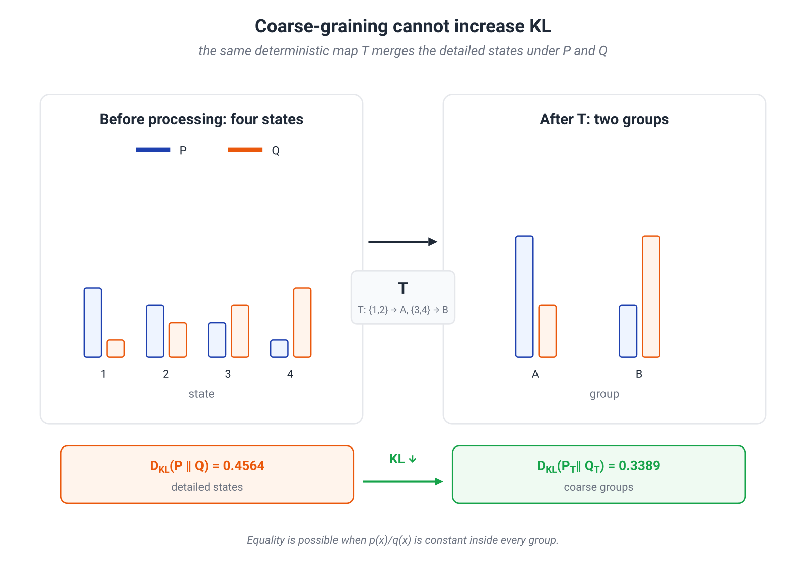
For

$$P=(0.4,0.3,0.2,0.1), \qquad Q=(0.1,0.2,0.3,0.4),$$

we have

$$D(P\|Q)\approx0.4564\ \text{nats}.$$

Merge the first two states and the last two states:

$$\bar P=(0.7,0.3), \qquad \bar Q=(0.3,0.7).$$

Now

$$D(\bar P\|\bar Q) \approx0.3389\ \text{nats}.$$

Distinguishability decreased because we can no longer see how probability mass is arranged inside each group.

The equality condition is particularly informative. KL is preserved exactly when the likelihood ratio

$$\frac{p(x)}{q(x)}$$

is constant within each group. Equivalently, whenever the group masses are positive,

$$P(X=x\mid Y=y) = Q(X=x\mid Y=y).$$

Once the group is known, the fine-grained state provides no additional evidence for distinguishing $P$ from $Q$. This is the exact algebraic form of the claim that a compression has lost nothing relevant to this distinction. The same pattern will later lead to the Data Processing Inequality and sufficient statistics.

For an arbitrary stochastic channel, the proof has the same shape: apply log-sum to the terms $p(x)K(y\mid x)$ and $q(x)K(y\mid x)$. In Module 5 this construction becomes the basis of data processing for mutual information.

4.6. One theorem, four working mechanisms

It is useful to collect the route in one table.

The important skill is not merely recognizing the word “Jensen” inside another proof. It is asking a transferable question:

What exactly is being averaged, which function is applied after the average, and what is the curvature of that function on the relevant domain?

This question prevents two opposite mistakes. The first is swapping operations as though nonlinearity were linear. The second is seeing convexity and drawing a much broader conclusion about the entire system. Jensen compares specific quantities in a fixed setup; generalization, optimization, and behavior under distribution shift require separate arguments.

The same machinery will return in richer forms:

• in Module 5, log-sum becomes data processing for KL and mutual information;
• in Module 8, equality conditions reappear alongside sufficient statistics and exponential families;
• in Module 9, the ELBO enters VAEs, the Information Bottleneck, and rate–distortion;
• in Module 11, convexity produces variational representations of divergences;
• in Module 12, KL appears as a complexity term in PAC-Bayes.

4.7. What to carry into ML practice

1. For convex $\phi$, $$\phi(\mathbb E X)\le\mathbb E\phi(X),$$ and the sign reverses for concave $\phi$.
2. The gap comes from both dispersion in the arguments and curvature of the function. Averaging identical predictions changes nothing.
3. Probability mixtures and mean logits define different ensembles. Both beat the average member under NLL, but neither dominates the other universally.
4. The ELBO is Jensen applied directly to the log marginal likelihood; its exact gap is $D_{\mathrm{KL}}(q(z\mid x)\|p(z\mid x))$.
5. Log-sum is a working form of KL nonnegativity. It explains joint convexity and why merging states cannot increase distinguishability.
6. Convexity gives an exact local guarantee about specified quantities. It does not replace checks of optimization, generalization, calibration, or target-distribution performance.

4.9. References and primary sources

• Boyd & Vandenberghe, Convex Optimization — convex functions, supporting hyperplanes, logsumexp, and Jensen's inequality.
• Cover & Thomas, Elements of Information Theory — the log-sum inequality, joint convexity of KL, and data processing.
• Kingma & Welling, Auto-Encoding Variational Bayes — the variational lower bound and amortized inference for models with continuous latent variables.
• Lakshminarayanan, Pritzel & Blundell, Simple and Scalable Predictive Uncertainty Estimation Using Deep Ensembles — practical context for averaging probabilistic predictions.
• Bregman, The relaxation method of finding the common point of convex sets and its application to the solution of problems in convex programming — the original Bregman-divergence construction.