Module 10. Algorithmic Information Theory: Shortest Descriptions, MDL, and Universal Prediction

How to read this module. Sections 10.1–10.8 form the main route. We first move from the average number of bits required by a source to the description length of one particular object, then connect that idea to Shannon entropy, universal prediction, MDL, and compression-based similarity. Sections 10.9–10.10 are optional second-pass discussions of AIXI and Landauer's principle.

10.1. From a distribution to one particular object

Consider three files of the same size: one million bits each.

• The first contains only zeros.
• The second contains the first million binary digits of $\pi$.
• The third was obtained from a physical source of randomness.

As stored bit strings, they have the same length. As descriptions, they are radically different. The first needs only an instruction such as “print one million zeros.” The second needs an algorithm for computing $\pi$ and the requested number of digits. The third will most likely have no description substantially shorter than the file itself.

This raises a question that does not begin with a probabilistic source:

How many bits are required to reproduce this particular object?

Algorithmic information theory (AIT) answers by looking for the shortest effective description: a program that prints the object and halts.

This is not a replacement for Shannon theory. It changes the level of analysis.

• Entropy begins with a distribution and asks for the average coding bill across possible messages.
• Algorithmic complexity begins with a specific string and asks for its shortest executable explanation.

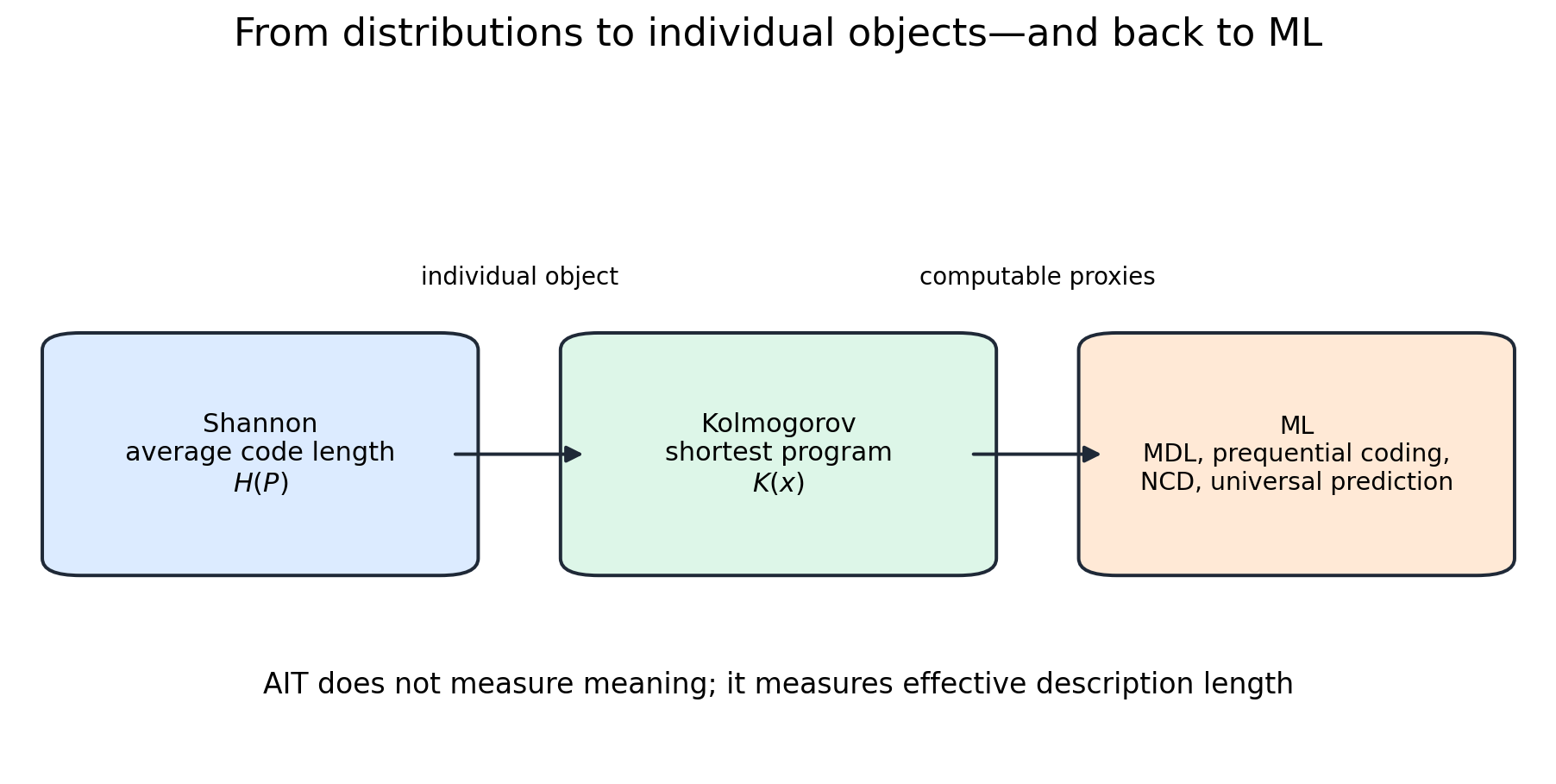
The distinction is useful in several ML settings.

Model selection. A larger model may reduce the data loss more strongly, but the model itself must also be paid for. This leads to the MDL account “model plus data given the model.”

Representation analysis. High probe accuracy does not tell us how easily a property can be extracted. A prequential code also charges for the number of examples and predictive bits required to learn the extraction rule.

Object similarity. If, after receiving $x$, the receiver needs only a short supplement to reconstruct $y$, the objects share algorithmic structure. A computable version of this idea leads to NCD.

Universal prediction. Giving shorter computable explanations greater prior weight produces an idealized predictor that competes with all computable models at once.

We should also set the boundary immediately. A short description can reveal regularity, but it does not measure meaning, truth, usefulness, or beauty. A very short program may print a meaningless string and may take an astronomical time to run. AIT measures descriptive complexity, not every interesting property of an object.

10.2. Kolmogorov complexity and the description language

The shortest program

A description is meaningful only together with a language that the decoder can execute. Fix a universal prefix machine $U$. Its halting programs are arranged so that no valid program is a prefix of another. This makes a stream of program bits uniquely decodable and lets program lengths behave like prefix-code lengths.

The prefix Kolmogorov complexity of a string $x$ is

$$\boxed{ K_U(x) = \min_{p:\,U(p)=x}|p| }.$$

It is the length of the shortest self-delimiting program that prints $x$ and halts.

The subscript $U$ is often omitted, but the machine remains part of the definition. The question is always: how concisely can the object be described in the chosen universal language?

A self-delimiting literal description

For plain complexity $C(x)$, a program can contain the string itself plus a fixed instruction to print the remaining bits. Hence

$$C(x)\le |x|+O(1).$$

A prefix program must tell the decoder where the length description ends and the string begins. A standard construction gives

$$\boxed{ K(x) \le |x|+K(|x|)+O(1) }.$$

For $n=|x|$, the cost $K(n)$ grows only logarithmically; for sufficiently large $n$, for example,

$$K(n) \le \log_2 n+2\log_2\log_2 n+O(1).$$

The overhead is small relative to a long string, but conceptually essential: self-delimitation is what makes weights of the form $2^{-|p|}$ compatible with a probability sum.

The invariance theorem

An immediate objection is that the same idea takes different numbers of bits in Python, C, and a Turing-machine language. Does complexity merely measure syntax?

Let $U$ and $V$ be two optimal universal prefix machines. There is a constant $c_{U,V}$, independent of $x$, such that

$$\boxed{ |K_U(x)-K_V(x)|\le c_{U,V} }.$$

The mechanism is simple. Machine $U$ can contain a fixed interpreter for $V$ and append any $V$-program to it. The interpreter cost is paid once and does not grow with the object.

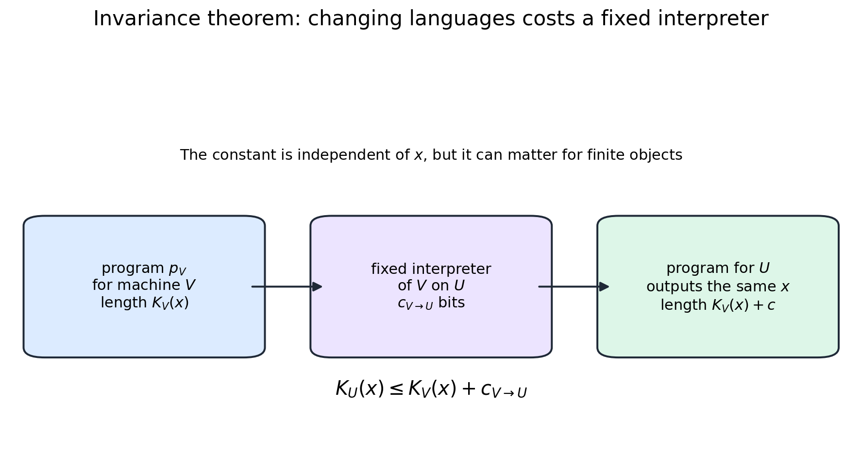
The theorem lets us discuss $K(x)$ up to an additive constant. For large objects this is a powerful form of robustness. For short strings, the compiler constant may be comparable to the quantity being measured, so the absolute value is not a machine-independent physical constant of the object.

Conditional complexity

If the decoder already knows an object $y$, define

$$\boxed{ K(x\mid y) = \min_{p:\,U(p,y)=x}|p| }.$$

This is the length of the shortest additional description of $x$ when $y$ is available as side information.

If $x$ and $y$ are two versions of a repository, $K(x\mid y)$ may be close to the length of a compact patch even when either repository is large on its own. This is the idea that will later become an algorithmic similarity measure.

What $K(x)$ measures

Strings of the same length can lie at very different points on the descriptive-complexity scale:

• a million zeros can be specified by a repeat count;
• a periodic string by a pattern and a repeat count;
• the first $n$ digits of $\pi$ by an algorithm and the value of $n$;
• a typical string of independent fair bits requires an almost literal description.

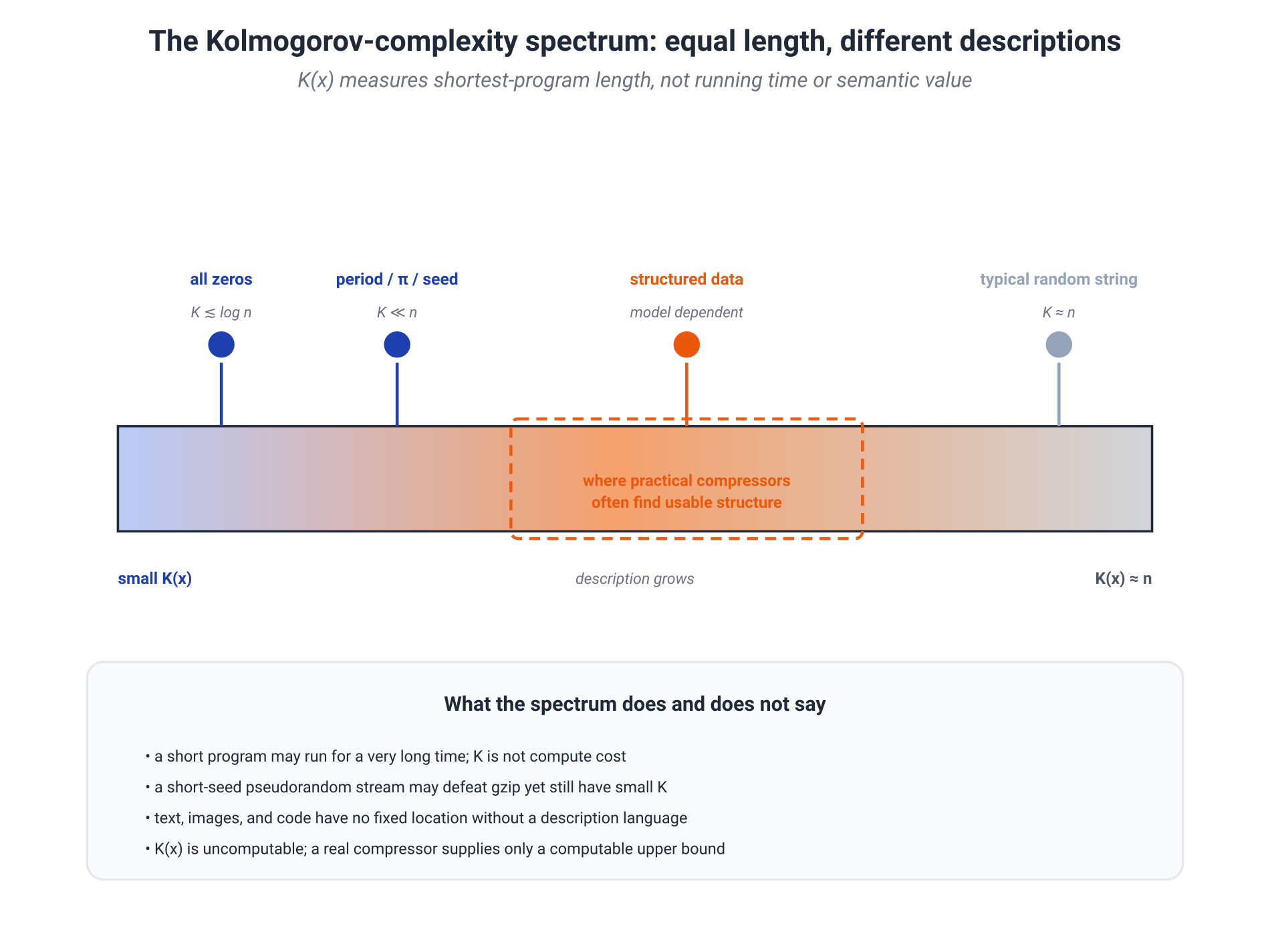
Program length must be kept separate from running time. A short program may take extremely long to compute its output. Conversely, a large weight file may produce outputs quickly. Kolmogorov complexity measures description length, not computational cost.

There is another useful surprise. A pseudorandom stream generated from a short program and a short seed has a concise algorithmic description, even though gzip may fail to compress it at all. A practical compressor searches for a restricted family of regularities; $K(x)$ minimizes over all programs.

10.3. Incompressibility, uncomputability, and real compressors

Why most strings cannot be compressed much

Consider all $2^n$ binary strings of length $n$. There are fewer than $2^{n-c}$ programs shorter than $n-c$. Each halting program prints at most one string. Therefore

$$\#\left\{ x\in\{0,1\}^n: K(x)<n-c \right\} < 2^{n-c}.$$

The fraction of strings compressible by at least $c$ bits is smaller than

$$\boxed{2^{-c}}.$$

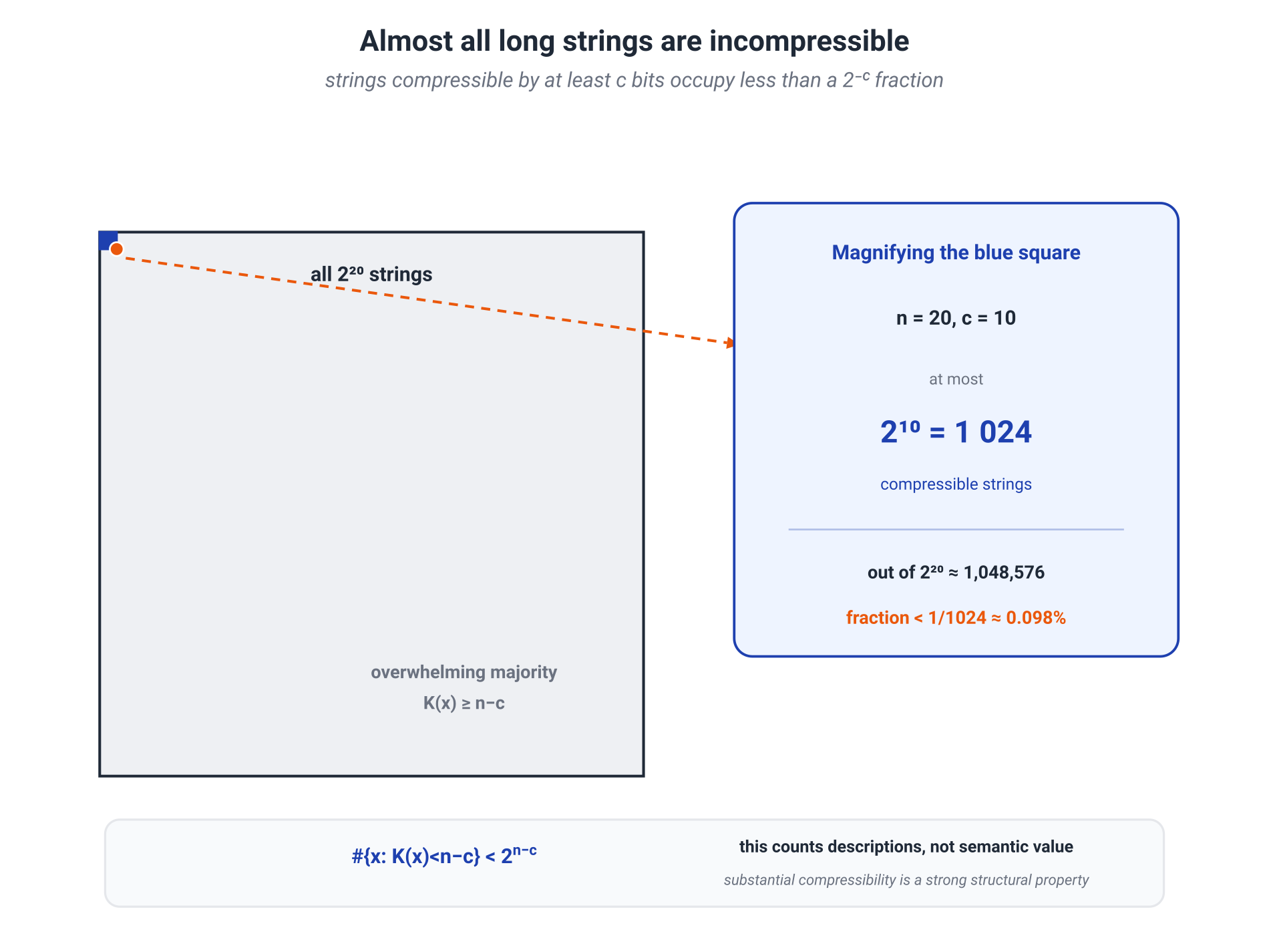
For example, fewer than about one in a million strings of any fixed length can be compressed by at least twenty bits. Structured objects occupy a tiny part of the space of all possible bit strings.

This is a counting statement about descriptions. It does not say that every incompressible string must look random to a human, and it says nothing about semantic value.

Why the ideal bill cannot be computed

Suppose an algorithm could compute $K(x)$ exactly. Given a number $m$, we could enumerate strings and find the first $x_m$ satisfying

$$K(x_m)>m.$$

But the program “receive $m$, find the first such string, and print it” has length

$$K(m)+O(1)=O(\log m),$$

which is far smaller than $m$ for large $m$. We would have produced a short description of an object constructed to have no short description. This is a contradiction.

Thus

$$\boxed{K(x)\text{ is uncomputable}.}$$

It is nevertheless upper semicomputable. We can dovetail more and more programs and lower our current upper bound whenever a shorter program for $x$ halts. What we cannot know is that the current candidate is already shortest: a still shorter program may halt after an unknown amount of time.

Uncomputability is not a performance problem that a faster processor will solve. It is part of the object being defined.

What gzip, zstd, and LZMA provide

Suppose a compressor outputs a string $C(x)$ and a fixed lossless decompressor reconstructs $x$. Then the program “run this decompressor on $C(x)$” yields

$$\boxed{ K(x) \le |C(x)|+c_C },$$

where $c_C$ pays for the decompressor, the format, and the input convention.

A real compressor therefore supplies a computable upper bound on $K(x)$. It does not supply a known approximation guarantee to the ideal value.

Poor compression can have several explanations:

1. the object is genuinely close to algorithmically incompressible;
2. its regularity lies outside the compressor's model class;
3. the file is too small and headers dominate;
4. the format or preprocessing hides useful structure.

A useful engineering interpretation is:

A compressor is an executable theory of regularity. Its code length reports which patterns that particular theory can exploit.

Mathematical note: randomness of an infinite sequence

For an infinite sequence, one long incompressible prefix is not enough. Martin-Löf randomness requires the sequence to pass every effective statistical test of measure zero. The Levin–Schnorr theorem links this definition to prefix complexity: a binary sequence $\omega$ is Martin-Löf random if and only if there is a constant $c$ such that

$$K(\omega_{1:n})\ge n-c$$

for every $n$. We will mainly work with finite objects, but this result shows why algorithmic randomness is not synonymous with “one archiver found no repetitions.”

10.4. The bridge to Shannon entropy

Shannon and Kolmogorov start from opposite sides.

• Shannon fixes a distribution $P$ and seeks the average code length.
• Kolmogorov fixes an object $x$ and seeks the shortest executable description.

For a computable source, however, the two bills meet on average.

Let $P$ be a computable distribution over finite strings, and let $K(P)$ denote the length of a program that computes its probabilities to the required precision. Then

$$\boxed{ H_2(P) \le \mathbb E_{X\sim P}[K(X)] \le H_2(P)+K(P)+O(1) }.$$

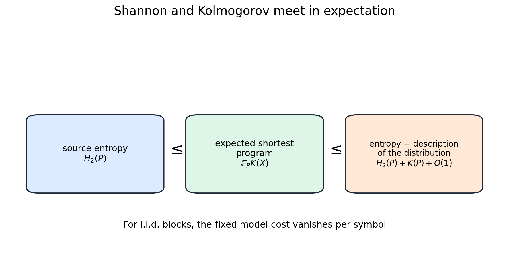
The lower bound

Choose one shortest prefix program for every $x$. These programs form a prefix code. The expected length of any prefix code is at least the entropy of the source, so

$$H_2(P) \le \mathbb E_P K(X).$$

The upper bound

We can transmit two things:

1. a program describing the distribution $P$;
2. a code for $x$ of length approximately $-\log_2P(x)$ bits.

Therefore

$$K(x) \le K(P)-\log_2P(x)+O(1).$$

Averaging turns the second term into entropy.

For an i.i.d. block $X_{1:n}$, a more explicit form is

$$H_2(X_{1:n}) \le \mathbb E K(X_{1:n}) \le H_2(X_{1:n})+K(P)+K(n)+O(1).$$

If the source is fixed and $H_2(X_{1:n})=nH_2(X)$, then

$$\frac1n\mathbb E K(X_{1:n}) \longrightarrow H_2(X).$$

The cost of specifying the source and the block length is spread across more and more symbols and vanishes per symbol.

This is the precise bridge:

Entropy is the typical average algorithmic complexity of long messages from a known computable source; $K(x)$ lets us discuss one object when no source has been fixed in advance.

The bridge does not erase the distinction. A single file does not determine a unique true distribution, and a short program that perfectly reproduces the training set need not predict new data well. Generalization depends on which part of the description transfers beyond the observed object.

10.5. Algorithmic probability and universal prediction

Programs as hypotheses

Prefix-freeness supports a useful thought experiment: flip a fair coin and read the resulting bits as a program. A program of length $|p|$ receives weight

$$2^{-|p|}.$$

By Kraft's inequality, the total weight of halting programs is at most one. Short programs receive greater prior weight, but long programs are not excluded.

For programs that print a finite string $x$ and halt, define the algorithmic probability

$$m_U(x) = \sum_{p:\,U(p)=x}2^{-|p|}.$$

Many programs may print the same string, so their weights are added. The coding theorem connects this sum to prefix complexity:

$$\boxed{ -\log_2m_U(x) = K_U(x)+O(1) }.$$

Equivalently,

$$m_U(x)\asymp2^{-K_U(x)}.$$

The shortest program determines the leading exponential scale, while the remaining programs add probability mass.

Predicting a continuation

For sequential prediction, it is cleaner to use a universal monotone machine that reads an infinite stream of fair random bits. Define $M(x)$ as the probability that its output begins with prefix $x$. Equivalently, sum the weights of the minimal input prefixes already sufficient to produce $x$:

$$\boxed{ M(x) = \sum_{p:\,p\text{ minimal and }U(p)\sqsupseteq x} 2^{-|p|} }.$$

Here $U(p)\sqsupseteq x$ means that the output begins with $x$; minimality prevents every extension of the same sufficient input prefix from being counted again.

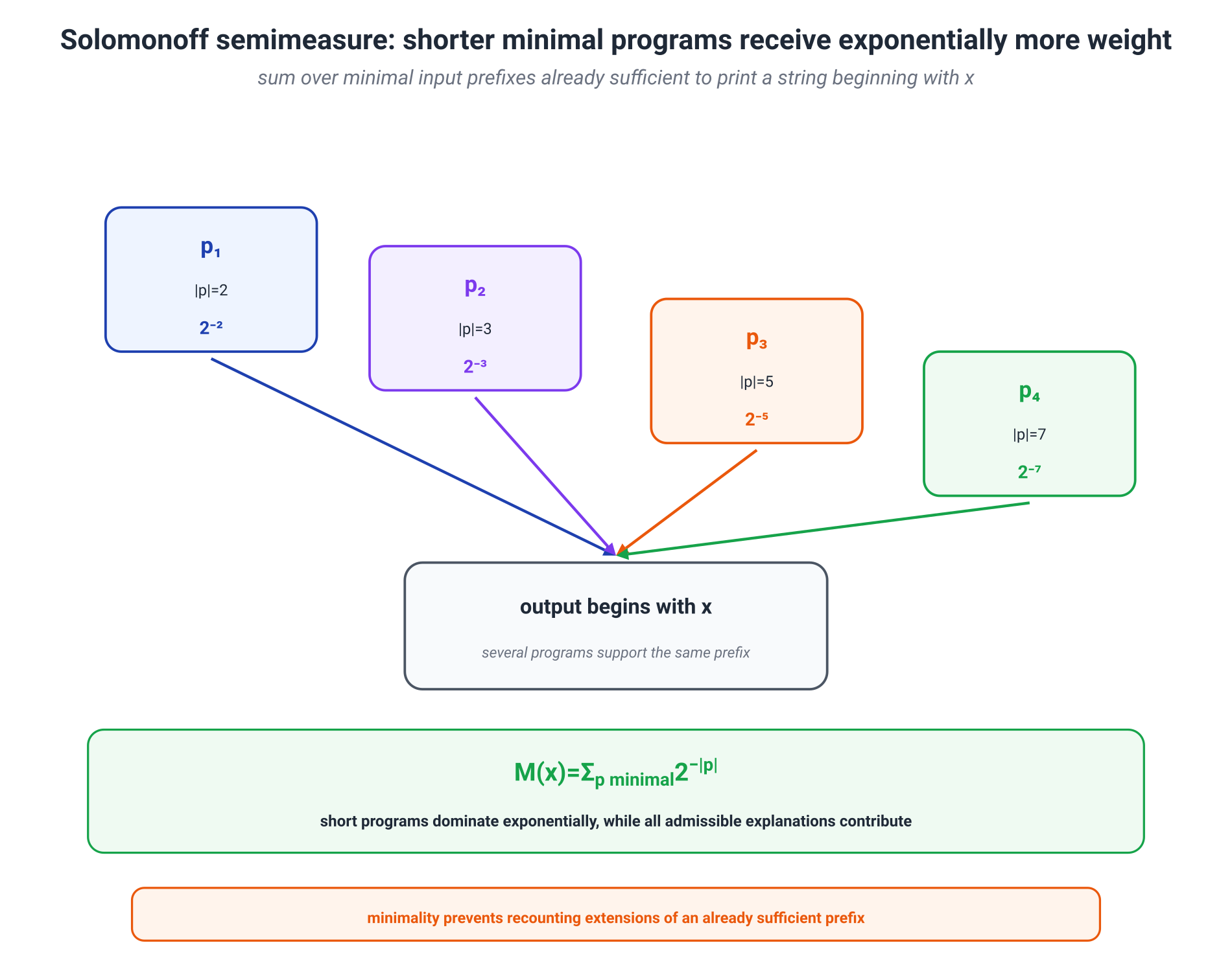
It is a semimeasure rather than an ordinary probability measure: some input mass may correspond to programs that stop after $x$ or fail to produce another symbol, so

$$M(x) \ge M(x0)+M(x1).$$

The ratios $M(xa)/M(x)$ provide conditional continuation weights; when needed, the outgoing mass can be normalized into a next-symbol distribution.

One technical distinction is worth naming once. The finite-output probability $m_U(x)$ is tied to prefix complexity $K_U(x)$. The sequential semimeasure $M(x)$ is naturally defined through a monotone machine and monotone complexity. The popular slogan “probability is about $2^{-K}$” conveys the shared idea, but formal theorems must keep the machine models separate.

Universal dominance

Let $\mu$ be a computable probabilistic source. The universal semimeasure contains a program that computes $\mu$, which implies

$$\boxed{ M(x) \ge 2^{-K(\mu)-O(1)}\mu(x) }$$

for every finite prefix $x$.

Taking negative logarithms gives

$$-\log_2M(x) \le -\log_2\mu(x)+K(\mu)+O(1).$$

This is best read as a coding bill:

The universal predictor pays for not knowing a computable source only once—through the source's description length—rather than paying a linear penalty as data accumulate.

For sequential conditional predictions, the likelihood ratio decomposes over time. In expectation, the cumulative conditional KL gap between the true predictor $\mu$ and a normalized Solomonoff predictor is bounded on the order of $K(\mu)$ bits. Consequently, for every fixed computable source, the average excess log loss per step tends to zero.

This is one of the module's strongest ideas. Occam's razor and Bayesian model averaging become a single construction: short computable explanations receive greater initial mass, and observations redistribute that mass among them.

Why this is not a practical algorithm

Computing $M(x)$ exactly would require knowing which programs will eventually print the requested prefix. That again runs into the halting problem. The universal semimeasure is lower semicomputable, but it is not computable as an ordinary function.

Its prior weights also depend on the selected universal machine. The invariance theorem controls this dependence by an additive constant in complexity, but for short data and prior-sensitive decisions that constant can matter.

Solomonoff induction is therefore not an architecture waiting to be implemented. It is a normative limit: sequential prediction as it would look if we could perform Bayesian averaging over all computable explanations with an algorithmic preference for shorter programs.

10.6. MDL in machine learning

The uncomputability of $K(x)$ does not invalidate the short-description idea. It changes the engineering task: instead of an unavailable ideal language, we design a concrete code and compare models within it.

The Minimum Description Length principle (MDL) says:

Prefer the model that yields the shortest complete description of the data.

A two-part code: model and residual

For a hypothesis $h$ and data $D$, the simplest account is

$$\boxed{ L(D,h) = L(h)+L(D\mid h) }.$$

The first term pays for the model. The second pays for whatever remains to be transmitted after the model is known.

Suppose model $A$ costs $100$ bits and codes the data in $1200$ bits. Model $B$ costs $300$ bits but reduces the data code to $850$ bits. Looking only at fit, $B$ gains $350$ bits; after paying for the model it still wins:

$$L_A=1300, \qquad L_B=1150.$$

If a probabilistic model assigns probability $p_h(D)$ and a matching entropy coder is used, then

$$L(D\mid h) \approx -\log_2p_h(D).$$

MDL turns the fit–complexity trade-off into accounting in a common unit rather than leaving it as a metaphor.

Codes, priors, and regularization

For a discrete model class, a prior $\pi(h)$ induces prefix lengths

$$L(h)=-\log_2\pi(h).$$

Minimizing

$$-\log p_h(D)-\log\pi(h)$$

then coincides with MAP model selection, up to the logarithm base.

Continuous parameters require more care. A prior density depends on coordinates and a base measure, while an exact real number cannot be sent with finitely many bits. One must specify parameter precision, integrate the parameters out in a one-part code, or use another universal coding construction.

This gives regularization a precise but limited interpretation. A Gaussian prior in a fixed Euclidean parameterization produces a quadratic MAP penalty. That is a useful connection, not a proof that every use of weight decay is the canonical description length of a neural network. A code must be specified rather than implied.

Prequential coding

A model need not be transmitted as a separate file. Sender and receiver can agree on the same learning algorithm and encode labels in blocks.

1. The first labels are sent with a simple baseline code.
2. Both parties train on the examples already transmitted.
3. The next block is encoded with the model's predictive probabilities.
4. After the block arrives, the model is retrained and the process repeats.

The total length is the sum of sequential log losses:

$$\boxed{ L_{\mathrm{preq}} = L(y_{1:n_0}) + \sum_j - \log_2 q_{\theta(D_{<j})} (y_{B_j}\mid x_{B_j}) }.$$

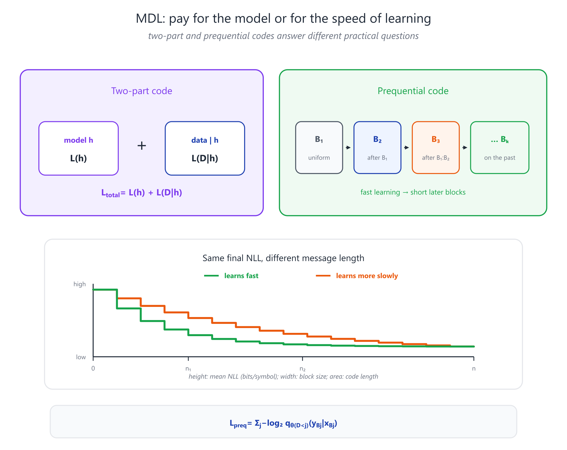
This code measures not only final performance but also learning speed. Two representations may allow the same classifier to reach the same eventual accuracy. If one requires a hundred examples and the other requires a thousand, the first produces a shorter prequential message.

That is the motivation behind MDL probing. The question “can a powerful classifier extract this property?” becomes “how many bits are needed to transmit the labels using this representation and a fixed learning protocol?” Voita and Titov study online and variational codes as practical estimators of this bill.

What an MDL result means

MDL does not eliminate modeling choices; it makes them explicit. A comparison depends on

• the code for the model class;
• parameter precision;
• the learning algorithm;
• data order and block boundaries in a prequential code;
• which metadata and protocol costs are included.

This does not make the result arbitrary. If the code and protocol are fixed before the comparison, message length is an exact reproducible quantity for that setup. The proper conclusion is not “this model is objectively simpler in every sense,” but “under the stated code, it gives a shorter complete description of these data.”

10.7. Similarity through joint compression

If $x$ and $y$ share structure, knowing one should shorten the description of the other. Conditional complexity turns this idea into a distance.

The ideal normalized information distance (NID) is

$$\operatorname{NID}(x,y) = \frac{ \max\{K(x\mid y),K(y\mid x)\} }{ \max\{K(x),K(y)\} }$$

up to the standard small corrections in conditional descriptions and normalization. It is small when either object can be reconstructed concisely from the other and near one when they share little algorithmic structure.

Because $K$ is uncomputable, practical work substitutes code lengths from a particular compressor $C$:

$$\boxed{ \operatorname{NCD}_C(x,y) = \frac{ C(xy)-\min\{C(x),C(y)\} }{ \max\{C(x),C(y)\} } }.$$

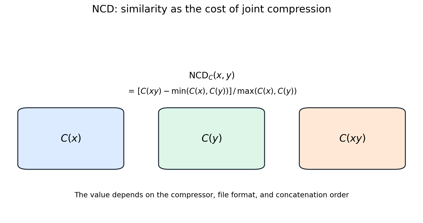
For example, if

$$C(x)=1000, \qquad C(y)=900, \qquad C(xy)=1300$$

bytes, then

$$\operatorname{NCD}_C(x,y) = \frac{1300-900}{1000} =0.4.$$

After paying for the shorter object, the joint message needs a relatively modest supplement.

Real compressors can be sensitive to concatenation order, so implementations often compare $C(xy)$ and $C(yx)$ and use their minimum or average. Headers and compressor imperfections can also push a measured NCD slightly outside the ideal range $[0,1]$.

What NCD actually sees

NCD does not require a manually designed feature space. If the compressor detects a shared dictionary, repeated fragments, similar syntax, or another reusable regularity, the joint code becomes shorter. The principle has been applied to texts, genomes, music, and other sequences.

A computable NCD inherits the inductive bias of its compressor:

• a dictionary coder for text and an image codec expose different patterns;
• short files are sensitive to headers;
• format and preprocessing change the result;
• concatenation order may introduce asymmetry;
• computable NCD does not automatically inherit every universality property of uncomputable NID.

NCD is therefore useful as a feature-free baseline and exploratory tool, but it still needs task-level validation and comparison with meaningful alternatives.

10.8. LLMs and universal prediction

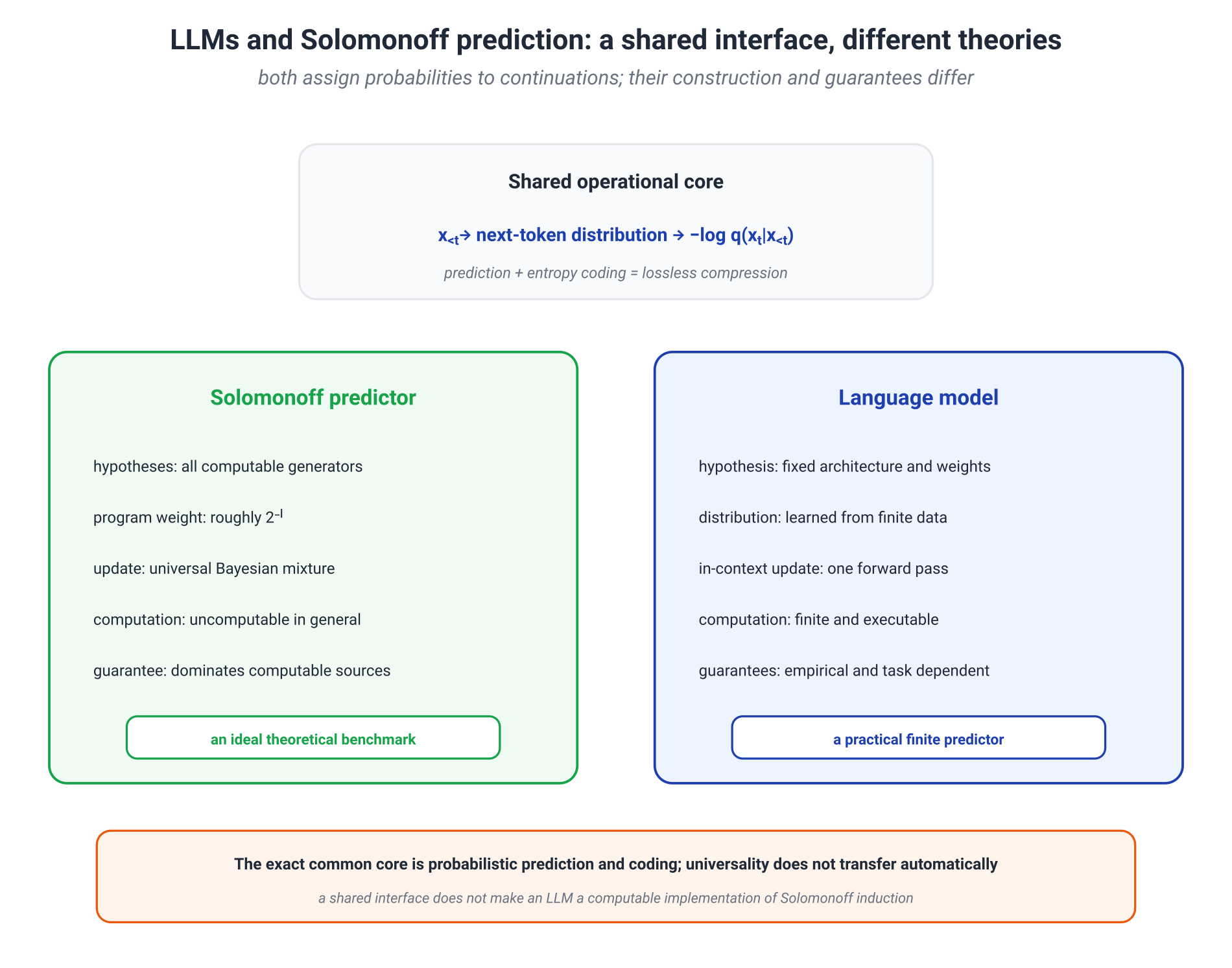
An LLM and a Solomonoff predictor belong on the same conceptual map: both assign probabilities to sequence continuations. They occupy very different points on that map.

The exact common core

For fixed weights, tokenizer, and context, a language model defines a computable distribution

$$q_\theta(x_t\mid x_{<t}).$$

Feeding those probabilities to an arithmetic or range coder produces a reversible compressor. Thus

$$\boxed{ \text{probabilistic prediction} + \text{entropy coding} = \text{lossless compression} }$$

is an exact operational statement. Language Modeling Is Compression demonstrates that large predictive models can in fact be evaluated as compressors across data modalities; as discussed in M6, a self-contained archive must also pay for the model and protocol.

The conceptual connection

Solomonoff induction averages all computable explanations, weighting them by program length. An LLM implements one large finite distribution learned from finite data by a particular optimization procedure.

Even so, its parameters can store many regularities, and context can select among them without changing the weights. In specific generative settings, in-context learning can indeed be derived as implicit Bayesian inference over a latent task. Xie and colleagues prove such a mechanism for a structured mixture of hidden Markov models.

This suggests a useful interpretation: the context acts as data, and the model's prediction acts like an approximate posterior predictive distribution. The theorem's scope, however, is determined by the structure of the pretraining distribution and task family.

Where the correspondence ends

A standard LLM

• has a finite architecture and a finite number of parameters;
• is trained on a finite dataset;
• uses a particular tokenizer and a bounded context;
• does not sum over all computable semimeasures;
• does not inherit universal dominance guarantees;
• may be miscalibrated and confidently wrong under distribution shift.

The most accurate statement is therefore:

An LLM is a computable sequential predictor and a potential compressor. Solomonoff induction is an uncomputable universal reference point for discussing prior breadth and adaptation, not an equivalent description of a particular LLM.

This boundary does not make the comparison useless. It identifies the exact common core—conditional probabilities and entropy coding—and separates it from properties that a finite learned model does not receive automatically.

Good compression of a chosen data representation is evidence of good probabilistic modeling of that representation. By itself, it is not a certificate of understanding, factual truth, or a causal world model.

10.9. Mathematical deepening: AIXI

A predictor answers “what will happen next?” An agent must additionally decide what to do.

AIXI combines

1. a universal Bayesian mixture over lower semicomputable chronological environment semimeasures, a class that includes computable environments;
2. sequential planning that maximizes expected reward.

Schematically, after history $h_{<t}$, the agent selects

$$a_t \in \arg\max_a \mathbb E_\xi \left[ \sum_{k=t}^{\infty}\gamma_k r_k \middle| h_{<t},a_t=a \right],$$

where $\xi$ is a universal environment mixture and $\gamma_k$ specifies the horizon or discounting.

What the construction contributes

AIXI cleanly separates three questions that are easy to conflate in a practical agent:

• which worlds are considered possible;
• how predictions are updated after observations;
• how predictions become actions through a reward function.

It is therefore useful as a normative blueprint for universal Bayesian reinforcement learning. It shows how algorithmic probability could enter not only prediction but decision making.

Why it is not an upper bound on intelligence

AIXI is incomputable. Its behavior also depends on the chosen universal machine, environment class, reward specification, and planning horizon. There is no AIXI invariance theorem guaranteeing that all reasonable universal priors lead to practically equivalent agents.

Some classical optimality properties are weaker than their informal names suggest. In the class of all computable environments, every policy can be Pareto-optimal in an overly broad sense; self-optimization is available only for environment classes that admit self-optimizing policies. Leike and Hutter show that an unfortunate universal-machine choice can change the agent's behavior drastically.

AIXI is best read as an idealized mathematical decomposition of a universal agent, not as a practical algorithm or a machine-independent maximum of possible intelligence.

10.10. Optional physical bridge: Landauer's principle

Algorithmic description length and the physical energy used by a computation are different quantities. Their thermodynamic connection enters through logically irreversible operations.

Consider a symmetric one-bit memory that is equally likely to contain $0$ or $1$ before erasure. An erase operation maps both inputs to a standard zero:

$$0\mapsto0, \qquad 1\mapsto0.$$

The input cannot be recovered from the output, so the operation is logically irreversible. In the isothermal quasistatic limit at temperature $T$, the minimum average heat transferred to the environment by this erasure is

$$\boxed{ Q_{\min}=k_BT\ln2 }.$$

At $T\approx300\,\mathrm K$,

$$Q_{\min} \approx 2.87\times10^{-21}\ \mathrm J.$$

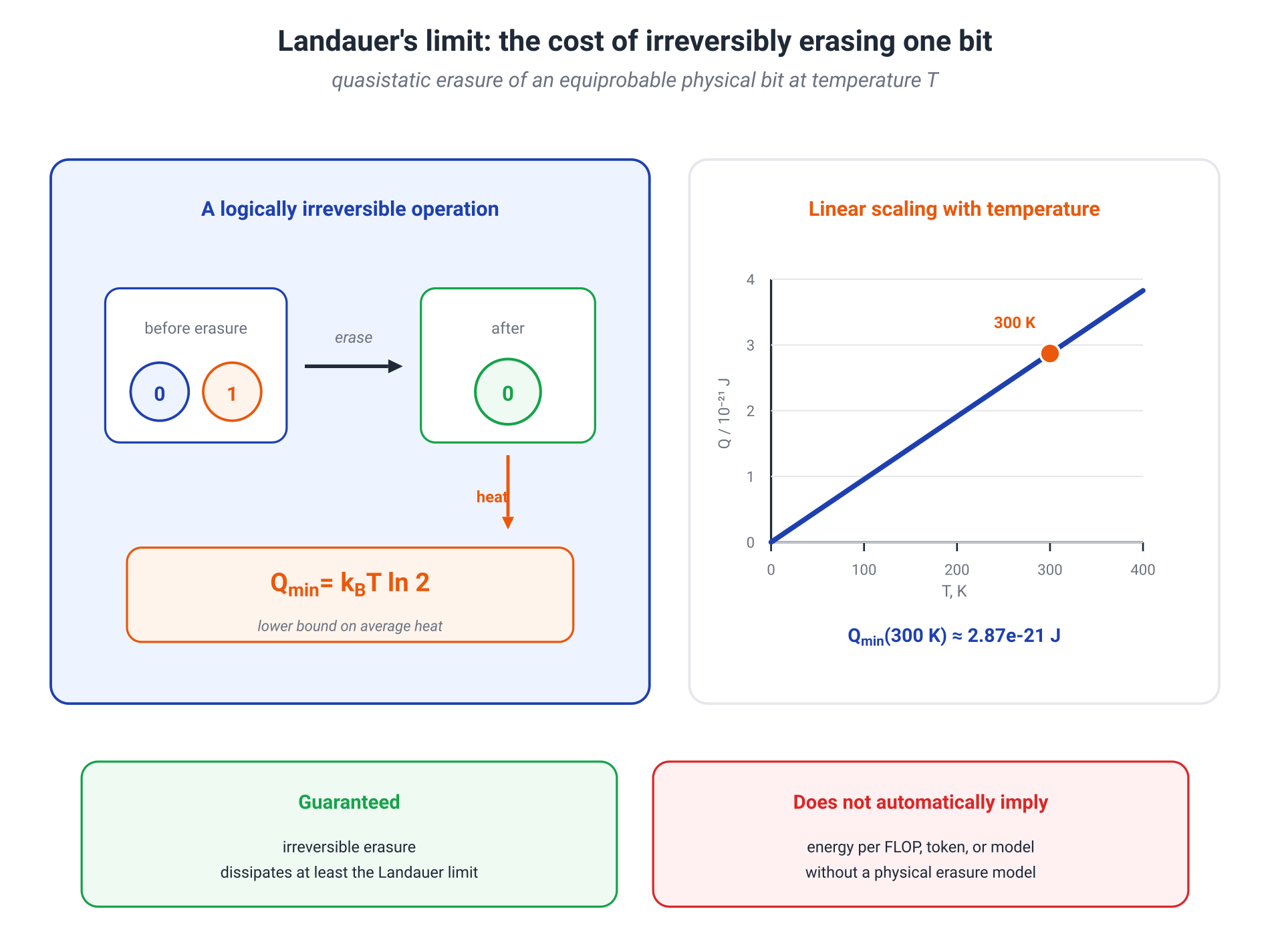
Landauer tied this lower bound specifically to logical irreversibility. Bérut and colleagues implemented a one-bit memory using a colloidal particle and observed the mean dissipated heat approach the Landauer limit for slow erasure protocols.

The formula is easy to apply too directly. One cannot estimate the energy of an LLM token by multiplying $k_BT\ln2$ by the number of FLOPs. Such a calculation would first have to identify

• which physical states encode logical bits;
• where information is irreversibly erased;
• the costs of memory and communication;
• leakage, clocking, and control losses;
• the distance from the reversible quasistatic regime.

Logically reversible computation need not pay the Landauer cost at every logical step. A finite-speed physical system still pays for noise control, synchronization, communication, and device imperfections.

It is useful to keep four accounts separate:

• $K(x)$: shortest-program length;
• computational complexity: time and memory;
• the Landauer limit: minimum thermodynamic cost of a specified erasure;
• accelerator energy: a property of particular hardware and workload.

10.12. What to retain

Algorithmic information theory changes the opening question. Instead of asking “how many bits does this source require on average?” it asks:

What is the shortest effective description of this object?

The central quantity is prefix Kolmogorov complexity,

$$K(x) = \text{the length of the shortest self-delimiting program for }x.$$

A single line of thought follows from it.

1. Most long strings are incompressible. There are simply not enough short programs to describe a substantial fraction of all strings.
2. The ideal complexity is uncomputable. Real compressors supply executable upper bounds and expose their own families of regularity.
3. Shannon and Kolmogorov agree on average. For a computable source, expected $K$ matches the entropy bill plus the cost of describing the source.
4. Algorithmic probability turns shortness into prior weight. A universal mixture pays once for a computable source description and then competes with it in sequential log loss.
5. MDL makes the idea operational. A “model plus data given the model” code compares fit, complexity, and learning speed in bits.
6. Joint compression induces similarity. NCD is useful when the selected compressor can expose shared structure.
7. An LLM lies on the same prediction-and-compression map but is not Solomonoff induction. The exact shared core is conditional probability plus entropy coding; universal guarantees do not transfer automatically.

The key engineering habit is:

Whenever an object is called simple or complex, ask which description language, decoder, precision, computational resources, and costs are being counted.

Primary sources

1. A. N. Kolmogorov, Three Approaches to the Quantitative Definition of Information, 1965.
2. R. J. Solomonoff, A Formal Theory of Inductive Inference, Part I and Part II, 1964.
3. M. Li and P. Vitányi, An Introduction to Kolmogorov Complexity and Its Applications, 4th ed., 2019.
4. J. Rissanen, Modeling by Shortest Data Description, 1978; P. Grünwald, The Minimum Description Length Principle, 2007.
5. E. Voita and I. Titov, Information-Theoretic Probing with Minimum Description Length, 2020.
6. R. Cilibrasi and P. Vitányi, Clustering by Compression, 2003/2005.
7. M. Hutter, Universal Artificial Intelligence: Sequential Decisions Based on Algorithmic Probability, 2005.
8. J. Leike and M. Hutter, Bad Universal Priors and Notions of Optimality, 2015; On the Computability of AIXI, 2015/2018.
9. G. Delétang et al., Language Modeling Is Compression, 2023/2024.
10. S. M. Xie et al., An Explanation of In-context Learning as Implicit Bayesian Inference, 2021/2022.
11. R. Landauer, Irreversibility and Heat Generation in the Computing Process, 1961; A. Bérut et al., Experimental Verification of Landauer's Principle Linking Information and Thermodynamics, 2012.