Module 6. Source coding: from entropy to real bits

How to read this module. The main route is §§6.1–6.8: from probabilistic models and the Kraft inequality to arithmetic coding, the AEP, entropy rate, and language-model metrics. §6.9 is a mathematical deepening on universal sequential prediction. §§6.10–6.11 return to LLM evaluation and to a reproducible compression experiment.

6.1. Engineering setup: the probabilistic model and the entropy coder

In earlier modules, $-\log q(x)$ appeared mainly as a loss: the less probability a model assigned to an observation, the larger the penalty. We will now read the same quantity as a description length.

Suppose two models evaluate the same data fragment $x$ and return the following probabilities for that fragment:

$$q_A(x)=2^{-1200}, \qquad q_B(x)=2^{-1116}.$$

These are probabilities of the entire fragment, not of a single token. For an autoregressive model, each is a product of token-level conditional probabilities, so probabilities of long sequences are naturally extremely small.

Convert the probabilities into lengths:

$$-\log_2 q_A(x)=1200, \qquad -\log_2 q_B(x)=1116.$$

Model $B$ therefore has a negative log-likelihood smaller by

$$1200-1116=84\ \text{ bits}.$$

Equivalently, model $B$ assigns the fragment an ideal information length that is 84 bits shorter. Producing a real reversible file still requires an entropy coder; its finite-precision and protocol overhead will be separated below.

The model and the coder have different roles.

A probabilistic model supplies next-symbol probabilities. An entropy coder uses those probabilities to construct a reversible bitstream.

Let a source generate $X_{1:n}$ from $P$, while an autoregressive model defines

$$q_\theta(x_{1:n}) = \prod_{t=1}^{n}q_\theta(x_t\mid x_{<t}).$$

The ideal information length of a particular sequence under the model is

$$\boxed{ L_{\mathrm{ideal}}(x_{1:n};q_\theta) = -\log_2q_\theta(x_{1:n}) = \sum_{t=1}^{n}-\log_2q_\theta(x_t\mid x_{<t}) }.$$

This is the familiar token-level negative log-likelihood, measured in bits. If a library reports NLL with natural logarithms, divide by $\ln 2$.

For example, if the model assigns three successive observations the conditional probabilities

$$\frac12, \qquad \frac18, \qquad \frac14,$$

then the ideal bill is

$$1+3+2=6\ \text{bits}.$$

The logarithm is doing the same job as in Module 1: it turns a product of conditional probabilities into an additive coding cost.

Ideal length, bitstream length, and total description length

A compression experiment has three relevant lengths.

1. Ideal data length $$L_{\mathrm{ideal}}=-\log_2q_\theta(x).$$ This is what bit-valued NLL measures.
2. Emitted bitstream length $$L_{\mathrm{stream}} =L_{\mathrm{ideal}}+L_{\mathrm{coder\ overhead}}.$$ Finite probability precision, termination, headers, and alignment live here.
3. Total self-contained description length $$L_{\mathrm{total}} =L(\theta)+L(\text{tokenizer})+L(\text{coder/protocol}) +L_{\mathrm{stream}}+L(\text{metadata}).$$ This is the relevant bill when the decoder does not already possess the model and protocol.

A validation loss measures the first ledger. A practical range coder approximates the second. A standalone archive must pay the third.

One more boundary will matter throughout the module. Entropy lower-bounds an expected length under a specified source. It does not forbid an individual regular string from being much shorter than the average. A million zeros may be exceptionally cheap; the theorem says that no lossless method can systematically push the mean length below the source entropy.

6.2. Prefix codes and the Kraft--McMillan inequality

Begin with the simplest code: assign a binary string to every symbol in a finite alphabet

$$\mathcal X=\{x_1,\ldots,x_m\}.$$

A code is prefix-free if no codeword is the beginning of another. Thus

$$\{0,10,110,111\}$$

is prefix-free, whereas

$$\{0,01,11\}$$

is not: after reading a zero, the decoder cannot know whether a symbol ended or the word 01 began.

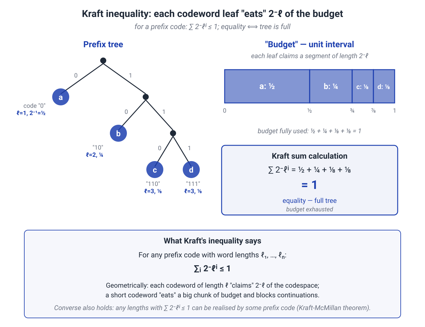
Prefix-freeness gives instantaneous decoding without separators. The convenience comes with a strict budget.

Kraft's theorem. Positive integers $\ell_1,\ldots,\ell_m$ are the lengths of some binary prefix code if and only if

$$\boxed{ \sum_{i=1}^{m}2^{-\ell_i}\le1 }.$$

Why the Kraft inequality arises

Read the full binary tree as one unit of resource. A codeword of length $\ell$ occupies a fraction

$$2^{-\ell}$$

of all sufficiently long binary continuations. Short words are expensive: length 1 immediately consumes half the tree; length 2 consumes one quarter; length 3 consumes one eighth.

For

$$\{0,10,110,111\},$$

the entire budget is used:

$$\frac12+\frac14+\frac18+\frac18=1.$$

Making a frequent symbol shorter requires reserving a large branch and pushing other symbols deeper into the tree.

This is why an arbitrary collection of short codewords cannot exist. Kraft's inequality is not bookkeeping trivia; it is the geometry of a scarce resource.

The converse is constructive: whenever the lengths fit within the budget, leaves can be placed in the tree without overlap. The same necessary inequality holds for the larger class of uniquely decodable codes, as part of the Kraft--McMillan theorem. Prefix codes will be enough for us: they achieve the same average-length bound and are simpler to decode.

6.3. The one-symbol source-coding theorem

Let $X\sim P$, with

$$p_i=P(X=x_i),$$

and let symbol $x_i$ receive a codeword of length $\ell_i$. The expected length is

$$L=\sum_i p_i\ell_i.$$

How small can $L$ be?

Lower bound on average code length

Every binary prefix code satisfies

$$\boxed{L\ge H_2(P)}.$$

The short proof belongs in the main route because it exposes exactly where coding inefficiency comes from.

Set

$$Z=\sum_i2^{-\ell_i}\le1, \qquad q_i=\frac{2^{-\ell_i}}{Z}.$$

Then $Q=(q_i)$ is the distribution implicitly defined by the code lengths, and

$$\begin{aligned} L-H_2(P) &=\sum_i p_i\log_2\frac{p_i}{2^{-\ell_i}}\\ &=D_{\mathrm{KL},2}(P\|Q)-\log_2Z\\ &\ge0. \end{aligned}$$

Now read the identity in words:

$$\boxed{ L-H_2(P) = \underbrace{D_{\mathrm{KL},2}(P\|Q)}_{\text{the code is tuned to the wrong source}} + \underbrace{(-\log_2Z)}_{\text{part of the tree is unused}} }.$$

The proof is a coding ledger. The gap has two causes: the lengths behave as though the source were $Q$ rather than $P$, and the code may leave some Kraft budget idle.

Equality $L=H_2(P)$ requires both

$$Q=P \qquad\text{and}\qquad Z=1,$$

hence

$$p_i=2^{-\ell_i}.$$

Exact one-symbol equality is possible for dyadic distributions, for which every $-\log_2p_i$ is an integer.

Upper bound: the Shannon code

The ideal real-valued lengths

$$-\log_2p_i$$

use the Kraft budget exactly because $\sum_i p_i=1$. But a binary codeword cannot be 2.37 bits long. Round up:

$$\ell_i=\left\lceil-\log_2p_i\right\rceil.$$

Then

$$2^{-\ell_i}\le p_i,$$

so Kraft holds, while

$$\ell_i< -\log_2p_i+1.$$

Therefore some prefix code satisfies

$$\boxed{ H_2(P)\le L<H_2(P)+1 }.$$

The $+1$ is not a fundamental loss on every symbol. It is the price of integer lengths in a one-symbol code. In §6.5 we postpone the rounding to the end of a long block and divide the constant across many symbols.

A code built for the wrong model

Suppose data come from $P$, but lengths are built from a model $Q$:

$$\ell_Q(x)=\left\lceil-\log_2q(x)\right\rceil,$$

with $q(x)>0$ on the support of $P$. Then

$$H_2(P,Q) \le L_Q < H_2(P,Q)+1.$$

Since

$$H_2(P,Q)=H_2(P)+D_{\mathrm{KL},2}(P\|Q),$$

we obtain

$$\boxed{ H_2(P)+D_{\mathrm{KL},2}(P\|Q) \le L_Q < H_2(P)+D_{\mathrm{KL},2}(P\|Q)+1 }.$$

This makes the operational meaning of KL literal:

under ideal fractional coding, $D_{\mathrm{KL},2}(P\|Q)$ is the expected number of extra bits paid for using the wrong probabilistic model.

A one-symbol prefix code adds less than one further bit of integer rounding.

6.4. Huffman coding, arithmetic coding, and range coding

Two classical algorithms solve the same problem but round at different places.

Huffman coding rounds every symbol length. Arithmetic coding postpones rounding until the message is complete.

Huffman coding

Huffman's algorithm constructs an optimal binary prefix code for a known finite distribution.

1. Take the two least probable nodes.
2. Merge them into a node whose probability is their sum.
3. Repeat until one root remains.

For

$$P=(0.40,0.20,0.15,0.15,0.10),$$

one optimal code has lengths

$$(1,3,3,3,3),$$

and therefore

$$L=2.20\ \text{bits/symbol}, \qquad H_2(P)\approx2.1464\ \text{bits/symbol}.$$

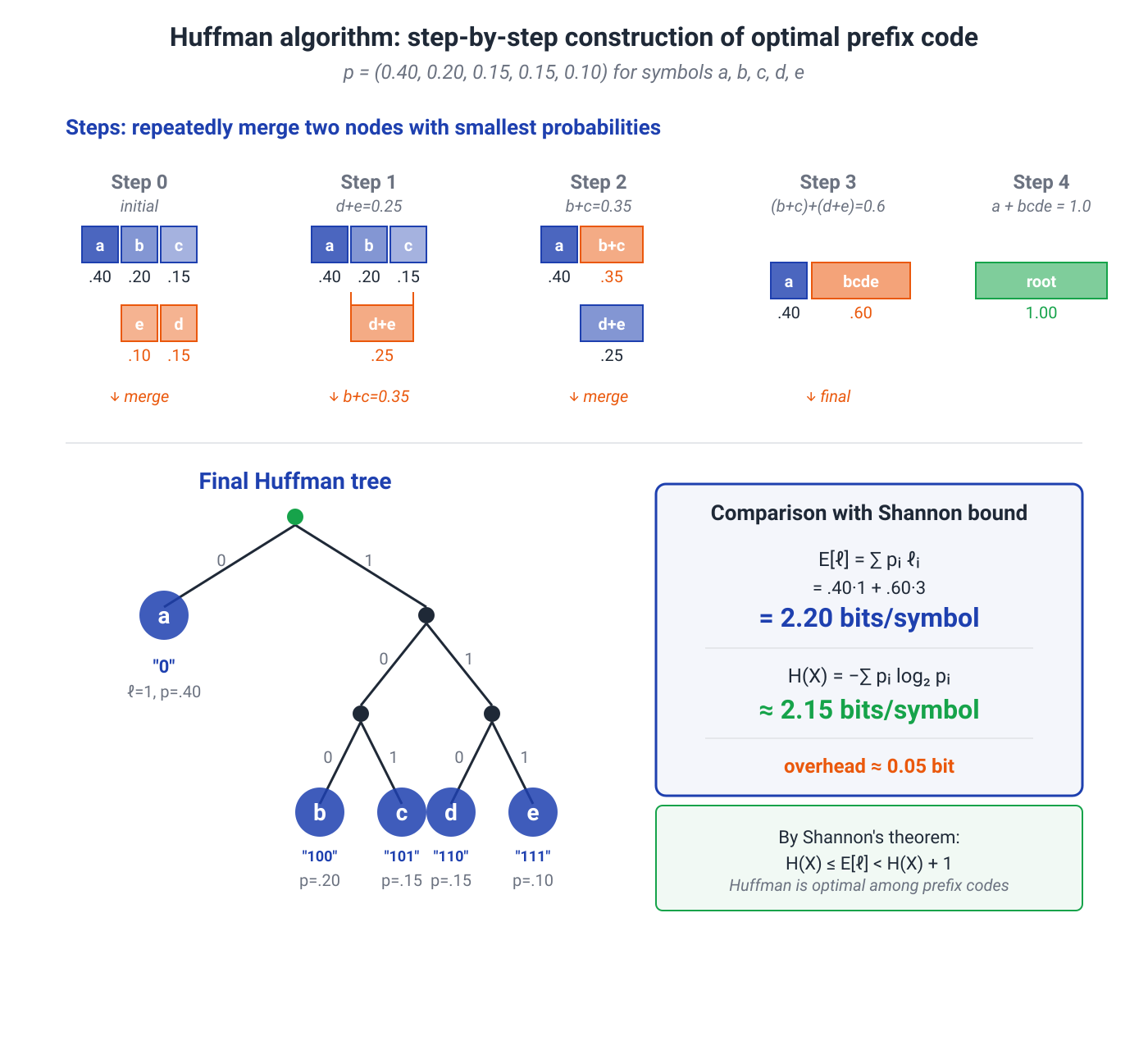
The gap is small. Integer granularity is much more visible for a highly skewed binary source:

$$P=(0.99,0.01).$$

Every nonempty binary one-symbol prefix code spends one bit per symbol, even though

$$H_2(P)=h_2(0.01)\approx0.0808.$$

This is neither a failure of Huffman coding nor a violation of Shannon's theorem. Huffman is optimal in its class; the class of one-symbol integer lengths is simply too coarse.

Arithmetic coding

Arithmetic coding does not give every symbol a separate word. It represents the entire sequence by a subinterval of $0,1)$.

Let

$$p(A)=0.5, \qquad p(B)=0.3, \qquad p(C)=0.2,$$

and partition $[0,1)$ as

$$A:[0,0.5), \quad B:[0.5,0.8), \quad C:[0.8,1).$$

For ACB, the interval evolves as

$$[0,1) \to[0,0.5) \to[0.40,0.50) \to[0.45,0.48).$$

Its final width is

$$0.03=p(A)p(C)p(B)=p(ACB).$$

![

The ideal information length is

$$-\log_2 0.03\approx5.06\ \text{bits}.$$

To terminate the code, however, we need more than a point inside $0.45,0.48)$. We need a finite binary prefix all of whose continuations stay in the target interval. The five-bit number

$$0.01111_2=\frac{15}{32}=0.46875$$

is inside the interval, but the prefix 01111 denotes the whole dyadic interval

$$\left[\frac{15}{32},\frac{16}{32}\right),$$

which extends past $0.48$.

The six-bit interval

$$\left[\frac{29}{64},\frac{30}{64}\right) = [0.453125,0.46875)$$

fits completely and corresponds to the prefix 011101.

This small detail matters: arithmetic coding transmits a finite binary description that keeps the decoder inside the intended interval, not merely a conveniently chosen real number.

A standard idealized construction can choose

$$\ell_{\mathrm{AC}}(x_{1:n}) \le \left\lceil-\log_2q(x_{1:n})\right\rceil+1 < -\log_2q(x_{1:n})+2.$$

Rounding is now paid once per message rather than once per symbol.

Conditional probabilities and autoregressive models

A fixed source partitions intervals with the same probability table at every step. A language model changes the table after every token:

$$q_\theta(x_t\mid x_{<t}).$$

After $n$ steps, the selected interval has width

$$\prod_{t=1}^{n}q_\theta(x_t\mid x_{<t}) =q_\theta(x_{1:n}),$$

and ideal length

$$-\log_2q_\theta(x_{1:n}) = \sum_{t=1}^{n}-\log_2q_\theta(x_t\mid x_{<t}).$$

That is the entire mechanism behind the language-modeling/compression correspondence: the model updates probabilities, and the coder updates an interval.

Practical systems often use range coding or Asymmetric Numeral Systems (ANS). Exact decoding requires encoder and decoder to reproduce the same

• quantized probabilities;
• tokenizer and vocabulary order;
• initial context, EOS convention, and reset rules;
• finite arithmetic and boundary handling.

The emitted stream is therefore close to the NLL length, but no single universal constant covers every implementation. Finite precision may accumulate a small redundancy; headers and metadata carry their own cost.

6.5. Long sequences: block coding, the AEP, and entropy rate

A one-symbol code is constrained by integer lengths. A long block spreads one unit of rounding across many symbols.

Lossless block coding

Let $X_1,\ldots,X_n$ be i.i.d. and treat the whole block $X^n$ as one supersymbol. Then

$$H(X^n)=nH(X).$$

Applying the one-symbol theorem to the block distribution gives a prefix code with

$$H(X^n)\le L_n<H(X^n)+1.$$

After dividing by $n$,

$$\boxed{ H(X) \le \frac{L_n}{n} < H(X)+\frac1n }.$$

This is a zero-error variable-length code: the block is recovered exactly, while the expected rate approaches entropy.

The phrase “entropy is achievable” now has a precise meaning. We do not create a 2.37-bit word for one symbol; we encode a long block and let fractional ideal lengths average out.

The AEP and concentration of per-symbol information

For a finite-alphabet i.i.d. source,

$$-\frac1n\log_2p(X^n) = \frac1n\sum_{t=1}^{n}-\log_2p(X_t) \xrightarrow{\mathrm{a.s.}} H_2(X).$$

This is the Asymptotic Equipartition Property (AEP).

Read it as follows: for a long random sequence, the sequence's own information length per symbol is almost surely close to entropy.

Define the typical set

$$A_\varepsilon^{(n)} = \left\{ x^n: \left|- \frac1n\log_2p(x^n)-H_2(X) \right|<\varepsilon \right\}.$$

For large $n$ it has three characteristic properties:

1. its probability is arbitrarily close to one;
2. each typical sequence has probability on the order of $2^{-nH_2(X)}$;
3. the number of typical sequences is on the order of $2^{nH_2(X)}$.

![

Thus there are exponentially many typical strings, each is exponentially unlikely, and together they carry almost all probability mass.

Indexing the typical set yields another source-coding statement: a fixed-rate code with rate just above $H(X)$ and error probability tending to zero. This is not the same as the previous zero-error variable-length construction. Atypical strings are either declared errors or handled by a separate escape mechanism.

Sources with dependencies

For text, the relevant quantity is not the entropy of an isolated token but the new uncertainty that remains after the past is known. For a stationary source, the natural rate is

$$h = \lim_{n\to\infty}\frac1nH(X_{1:n}),$$

when the limit exists.

For a finite-alphabet stationary ergodic source, the Shannon--McMillan--Breiman theorem gives

$$-\frac1n\log_2p(X_{1:n}) \xrightarrow{\mathrm{a.s.}} h.$$

It is $h$, not the marginal entropy $H(X_1)$, that governs asymptotic compression with dependencies. The marginal entropy ignores context and pays for the same predictable structure repeatedly.

6.6. Language-model metrics: PPL, BPC, and BPB

Perplexity, bits per character, and bits per byte are the same coding bill divided by different units.

Suppose a tokenizer maps text to $m$ tokens $t_{1:m}$. The average token NLL in bits is

$$\widehat L_{\mathrm{token}} = -\frac1m\sum_{i=1}^{m} \log_2q_\theta(t_i\mid t_{<i}).$$

Then

$$\operatorname{PPL} =2^{\widehat L_{\mathrm{token}}}.$$

Perplexity is an average code length with the logarithm exponentiated away.

A model spending 3 bits per token has PPL $2^3=8$. In the special uniform case this resembles eight equiprobable continuations. For a general distribution, it is better understood as the exponential of an average log price, not a literal candidate count.

Normalization per token, character, and byte

Token PPL depends on what counts as a token. If the same message probability is merely regrouped from six tokens into three pairs, total bits stay fixed but the average cost per new unit doubles.

For example, let

$$L_{\mathrm{total}}=12\ \text{bits}.$$

With six tokens,

$$2\ \text{bits/token}, \qquad \operatorname{PPL}_{\mathrm{token}}=4.$$

With three token pairs,

$$4\ \text{bits/pair}, \qquad \operatorname{PPL}_{\mathrm{pair}}=16.$$

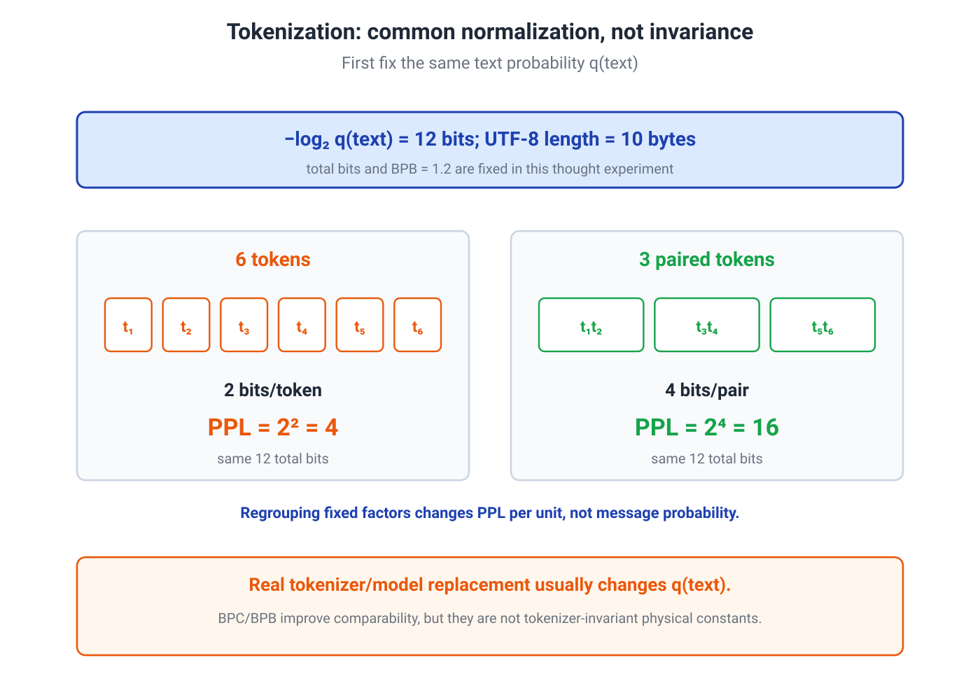
This is why token perplexities from different tokenizers are usually not directly comparable. Common denominators include

$$\operatorname{BPC} = \frac{-\log_2q_\theta(t_{1:m})}{N_{\mathrm{chars}}}$$

and

$$\operatorname{BPB} = \frac{-\log_2q_\theta(t_{1:m})}{N_{\mathrm{bytes}}}.$$

BPB is often easier to reproduce because bytes require only a fixed input file. BPC additionally depends on whether “character” means a byte, a Unicode code point, or a grapheme cluster.

Metric comparability and the role of tokenization

BPC and BPB do not remain unchanged when both tokenizer and model are replaced. A different tokenizer changes sequence length, vocabulary, computation, and usually the distribution $q_\theta$ itself.

The narrower statement is exact: if the probability of the same byte sequence is already fixed and we only regroup its factors, total bits and BPB remain unchanged, while PPL per new unit changes.

BPC/BPB therefore make comparisons more meaningful, but they do not remove the need for a protocol. The corpus, encoding, Unicode normalization, document boundaries, available context, and long-sequence evaluation method must still be fixed.

6.7. A language model as part of a compressor

Now assemble the full construction.

Encoder and decoder share

• model parameters;
• a tokenizer or another reversible input representation;
• the procedure for computing and quantizing probabilities;
• an entropy coder;
• start, stop, and context-reset rules.

The encoder observes the next symbol, obtains $q_\theta(\cdot\mid x_{<t})$, and narrows the interval. Having reconstructed the same prefix, the decoder computes the same distribution and determines which symbol the bitstream selected.

Under this protocol,

$$L_{\mathrm{stream}}(x_{1:n}) \approx -\log_2q_\theta(x_{1:n}),$$

and averaging over $P$ gives

$$\mathbb E_P[-\log_2Q_\theta(X)] = H_2(P)+D_{\mathrm{KL},2}(P\|Q_\theta).$$

Hence lower held-out log loss on the same distribution means a shorter expected data code.

There is an important engineering detail. If tokenization normalizes text irreversibly, the compressor recovers the normalized text rather than the original bytes. A genuine lossless archive needs a reversible representation or must separately encode the information discarded by preprocessing.

The Delétang et al. experiment

In Language Modeling Is Compression (ICLR 2024), pretrained models were coupled to arithmetic coding and applied to byte streams from text, images, and audio.

In Table 1, each dataset contains 1 GB and Transformer-based models process independent 2048-byte chunks. Chinchilla 70B obtains the following raw compression rates—compressed data-code size divided by raw size, excluding model weights:

• $8.3\%$ on enwik9;
• $48.0\%$ on grayscale ImageNet patches;
• $21.0\%$ on LibriSpeech.

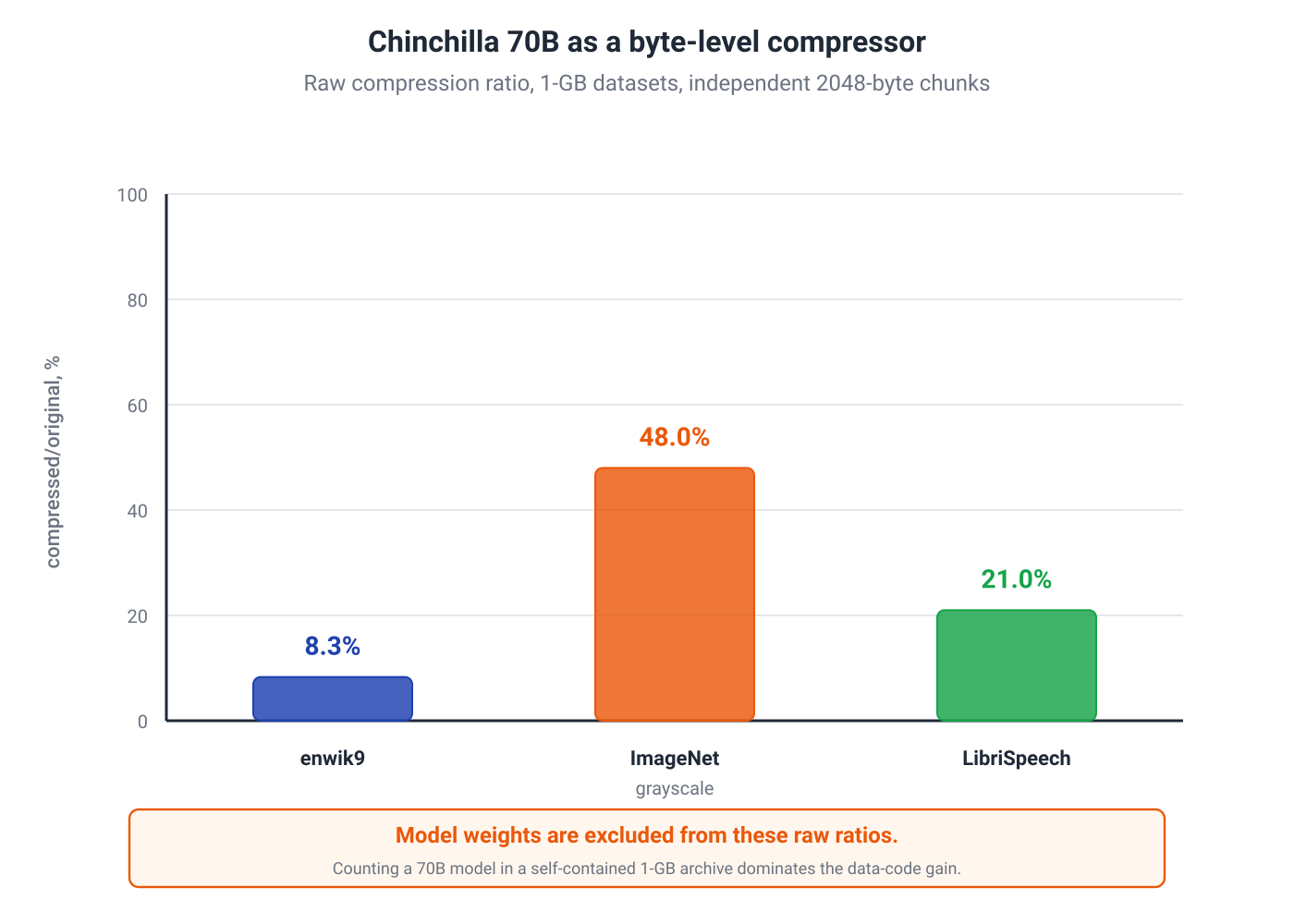
The result is genuinely striking: a model pretrained primarily on text assigns useful probabilities to non-text byte sequences as well.

The protocol also tells us exactly how far the claim reaches. It demonstrates byte-level predictive structure in particular 2048-byte chunks. It is not, by itself, evidence of semantic understanding of images or speech. And the raw ratio asks, “How short is the data code if both parties already possess the model for free?”

The paper's abstract reports somewhat better figures, $43.4\%$ and $16.4\%$, for ImageNet and LibriSpeech. To avoid mixing evaluation regimes, this module and its diagram use the explicit 2048-byte Table 1 values.

6.8. Model size, scaling laws, and total description length

Validation loss asks a useful question:

How many bits do the data need if the model is already available to both sides?

A standalone archive asks a stricter one:

Who pays for the model itself?

A two-part description has length

$$\boxed{ L_{\mathrm{two\mbox{-}part}}(\theta,x) = L(\theta)+L(x\mid\theta) }.$$

A larger model will often shrink the second term while increasing the first. For a fixed amount of data, an intermediate model size may minimize the total.

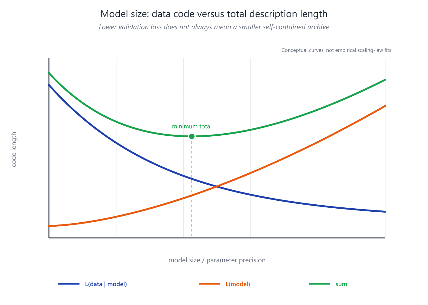
Delétang et al. charge neural-network weights at 2 bytes per parameter. Chinchilla 70B therefore costs roughly 140 GB before any data are coded. On a 1 GB enwik9 corpus, the data code is about $0.083$ GB, but the two-part total is approximately

$$140+0.083\ \text{GB},$$

which produces the table's adjusted compression rate of about $14008.3\%$.

This does not make large models useless. When one shared model serves an enormous stream of data, its cost can be amortized. It does mean that “Is this a good predictor?” and “Is this a good standalone archive for this dataset size?” are different questions.

Scaling laws and description length

When test cross-entropy falls with scale, the data-code length under an already shared model falls as well. This is an exact and useful reading of a scaling curve.

A stronger conclusion needs additional assumptions. A smooth power law alone does not imply

$$D_{\mathrm{KL}}(P\|Q_\theta)\to0$$

or guarantee that a fitted asymptote is the “true entropy of language.”

The reasons are ordinary:

• the model family may not contain the source;
• optimization may not find the best model in the family;
• a finite context window restricts the available conditional law;
• preprocessing and tokenization define a different problem;
• a held-out corpus is not a universal distribution over language;
• the empirical curve covers a finite range of scales.

The exact identity remains powerful:

$$H(P,Q_\theta) = H(P)+D_{\mathrm{KL}}(P\|Q_\theta).$$

But identifying an empirical asymptote with $H(P)$ requires a separate argument that the KL gap vanishes for the specified source and context regime.

6.9. Mathematical deepening: universal coding, sequential log loss, and ICL

Optional on a first pass. Here the “prediction = code” bridge is extended to an unknown source, where the predictor adapts along the sequence.

At time $t$, a sequential predictor outputs

$$q_t(x_t\mid x_{<t}).$$

Its cumulative bit-valued log loss is

$$L_n =-\sum_{t=1}^{n}\log_2q_t(x_t\mid x_{<t}).$$

This is also an ideal sequential code length. Online prediction under log loss and sequential compression use the same ledger.

A finite mixture of models

Suppose we have models $P_1,\ldots,P_K$ with prior weights

$$w_j>0, \qquad \sum_jw_j=1.$$

The Bayesian mixture is

$$Q(x_{1:n}) = \sum_{j=1}^{K}w_jP_j(x_{1:n}).$$

For every $j$,

$$Q(x_{1:n})\ge w_jP_j(x_{1:n}),$$

so

$$\boxed{ -\log_2Q(x_{1:n}) \le -\log_2P_j(x_{1:n}) + \log_2\frac1{w_j} }.$$

With a uniform prior, the mixture loses at most $\log_2K$ bits over the entire sequence relative to the best model in the finite class.

This is the clean idea behind universal prediction: uncertainty about which hypothesis will win is paid for by finite regret. The precise guarantee depends on the class. Lempel--Ziv, CTW, Bayesian mixtures, and other universal codes have different assumptions and redundancy rates; there is no assumption-free $O(\log n)$ guarantee for every source.

The connection to in-context learning and its limits

A prompt containing demonstrations changes the model's subsequent conditional distributions without changing its weights. Operationally, this resembles an adaptive sequential code: context improves prediction, and any log-loss reduction shortens the code.

Theory provides more specific mechanisms under explicit assumptions. Xie et al. derive implicit Bayesian inference for a pretraining distribution given by a mixture of HMMs. Hahn and Goyal connect emergent ICL to structural and compositional properties of the training distribution.

These results do not turn an arbitrary LLM into an optimal universal Bayesian predictor for every prompt. A measurable question is more modest:

How quickly does sequential log loss fall as relevant context is added, and relative to which comparator class is regret measured?

6.10. Compression quality and model capabilities

The implication

$$\text{better probabilistic prediction} \Longrightarrow \text{shorter lossless data code}$$

is mathematical. Moving from it to “the better compressor is more intelligent” requires a definition of capability and an evaluation protocol.

The Hutter Prize uses lossless compression of the fixed 1 GB enwik9 file as a test of discovering structure in a large text corpus. Under the official rules, the scored size includes not only compressed data but also the program that reconstructs them. The benchmark is therefore closer to total description length than to NLL with a free model.

Huang et al., in Compression Represents Intelligence Linearly (COLM 2024), compare 31 public base LLMs on 12 knowledge, coding, and mathematical-reasoning benchmarks. In their protocol, average benchmark score correlates with average BPC on external corpora at a Pearson coefficient of about $-0.93$.

That is a strong empirical signal: good modeling of external data can be a useful unsupervised capability metric. But the same paper shows that the relationship weakens when the compression corpus is poorly aligned with the evaluated domain. A later study of code models (Xuyang et al., 2025) reports a logarithmic rather than universally linear relationship under its protocol.

A defensible conclusion is therefore:

Held-out compression efficiency is a meaningful unsupervised measure of probabilistic modeling quality and may proxy some capabilities; the shape of that relationship depends on domain, model set, and benchmark, and it is not a general definition of intelligence.

Low BPC does not by itself certify factual truth, alignment, causal reasoning, robust planning, or safe behavior. That does not weaken the compression metric; it identifies the precise question the metric answers.

6.11. A practical protocol for evaluating an LLM as a compressor

Before publishing a statement such as “the model reaches 1.1 BPB,” write down the full agreement between encoder and decoder.

1. Input data. Exact file, version, license, and checksum.
2. Preprocessing. Encoding, Unicode normalization, line endings, and removed regions.
3. Unit. Bits/token, BPC, or BPB; for BPC, define “character.”
4. Tokenizer. Version, special tokens, and reversibility to the original bytes.
5. Boundaries. BOS, EOS, message length, and context resets.
6. Context policy. Independent chunks, sliding window, or continuous stream; every target must be counted exactly once.
7. Model. Exact revision, base or instruction-tuned variant, numerical precision, and evaluation mode.
8. Coder probabilities. How logits become integer frequencies and whether encoder and decoder reproduce them identically.
9. What was measured. NLL-equivalent length or an actually emitted bitstream.
10. Model cost. Whether weights and tokenizer are shared in advance or included in the archive.
11. Contamination. Whether the evaluation file may have appeared in pretraining.
12. Comparability. Whether every method received the same byte stream and the same available context.

Sliding-window evaluation of a causal LM has a common off-by-one trap. Library losses typically compare

$$\texttt{logits[:, :-1]} \quad\text{with}\quad \texttt{labels[:, 1:]},$$

so the number of scored targets should be checked after this shift. Otherwise a boundary token can be skipped or counted twice.

A good report separates

• NLL-equivalent bits;
• actual compressed-stream size;
• format and coder overhead;
• model cost, when included.

Then “the LLM compresses the data” is a reproducible engineering result rather than a metaphor.

6.13. Conclusion

At the beginning of the module, $-\log q$ was a familiar loss. It now has a physically testable meaning: it is the ideal bill, in bits, that a probabilistic model assigns to an observed sequence.

The central construction fits in one line:

$$\boxed{ \text{probabilistic model} + \text{entropy coder} = \text{lossless compressor} }.$$

Kraft's inequality explained why short codewords compete for a finite budget. Shannon's theorem decomposed coding redundancy into model mismatch and unused tree capacity. Huffman gave the best one-symbol prefix code, while arithmetic coding postponed rounding until the message ended. The AEP explained why long sequences acquire a stable per-symbol length, and entropy rate extended the picture to dependent sources.

For ML, the main consequence is particularly simple:

Lower held-out log loss means a shorter expected data code—under the same source, unit, and protocol.

Engineering honesty begins after that equality. PPL depends on the token; BPC and BPB require a common byte protocol; a real stream has coder overhead; a self-contained archive pays for the model; a strong compressor is a strong predictor but does not automatically receive a certificate of general intelligence.

The theory does not dissolve the beautiful link between prediction and compression. It strengthens it by identifying the exact equality, the exact price of mismatch, and the exact point where the rest of the system must be added to the data code.

Primary sources

• C. E. Shannon, A Mathematical Theory of Communication (1948).
• D. A. Huffman, A Method for the Construction of Minimum-Redundancy Codes (1952).
• T. Cover and J. Thomas, Elements of Information Theory, Chapter 5.
• G. Delétang et al., Language Modeling Is Compression, ICLR 2024.
• Y. Huang et al., Compression Represents Intelligence Linearly, COLM 2024.
• S. Xuyang, X. Luo et al., Is Compression Really Linear with Code Intelligence? (2025).
• S. M. Xie et al., An Explanation of In-Context Learning as Implicit Bayesian Inference, ICLR 2022.
• M. Hahn and N. Goyal, A Theory of Emergent In-Context Learning as Implicit Structure Induction (2023).
• M. Hutter, Human Knowledge Compression Contest—official enwik9 rules.