Module 1. Introduction

How to read this module. The required first pass is §§1.1–1.4. Section 1.3 uses formulas as a short bridge from probability to entropy and cross-entropy; §1.4 explains the route through the course. The overview and reference sections that follow are not meant to be read linearly. Sections 1.9–1.10 preserve the complete rigorous derivation of Shannon entropy for a second pass, preferably after Module 2 or Module 4.

Three courses, one program. “Information Theory for ML: From NLP and LLMs to CV and RL” provides the mathematical foundation of the series. Two independent companion courses develop the applied threads: “Modern LLMs” covers the architecture, training, inference, and evaluation of modern language models, while “Reinforcement Learning for LLM” develops feedback-based training, RLVR, and agentic systems. Each course can be taken independently: cross-references provide optional depth rather than replacing explanations needed to continue.

1.1. Information and meaning: why they are not the same thing

In 1948, Claude Shannon was not merely developing a theory of transmission over a telegraph wire. He was building a common language for sources, codes, and noisy channels. The engineering question was almost provocatively simple: what is the smallest resource needed to transmit a message reliably? Answering it required a way to measure uncertainty before the message arrived.

Start with the intuition. The statement “the sun will rise in Paris tomorrow” barely changes our expectations. “A tornado will hit Paris tomorrow,” if it turns out to be true, changes them sharply. The second event need not be more valuable, profound, or meaningful. It is simply much less probable under the chosen model of the world and is therefore more surprising.

This is the first nontrivial idea of the course: information and meaning are not the same thing. Shannon deliberately set semantics outside the boundary of his engineering problem. At first this sounds like abandoning the interesting part. In fact, the restriction made the mathematics possible: instead of debating the value of a message, we obtained probabilities, codes, compression limits, and channel capacity.

The move feels natural today, but it was conceptually radical. Nyquist and Hartley had already connected communication to the number of distinguishable messages and to a logarithmic scale. Shannon added probabilistic sources, unequal message probabilities, long sequences, and noise, then assembled them into one theory.

Keep this choice in mind; it will echo through the course. A probabilistic language model can be converted into a lossless compressor, and its negative log-likelihood is connected to code length. But good text compression is not identical to text understanding; a low loss is not a certificate of truth; and “the entropy of language” becomes a precise phrase only after a source model and the relevant long-sequence regime have been specified. Shannon's framework is powerful not because it measures everything, but because it measures one layer of the problem with unusual precision.

Three questions that are enough to distinguish in words for now

Later we will introduce three closely related but different quantities:

• how surprising this particular realized outcome is;
• how uncertain the source is on average before observation;
• how much observing one variable reduces uncertainty about another on average.

Ordinary language may call all three “information.” Mathematically they become different objects: surprisal, entropy, and mutual information. Their formulas will appear where they begin to explain something—the first two in Module 2 and the third in Module 5. At this point, distinguishing the questions matters more than memorizing notation.

1.2. The Shannon frame: strength and limitations

The Shannon frame is useful precisely because it answers a restricted family of questions. Let us first see what that restriction buys us, then mark the exact boundary of the claim.

Where the Shannon frame is productive

Training language models. Cross-entropy gives a clear task: the model distribution should assign high probability to observed continuations. That makes cross-entropy, perplexity, and bits per token meaningful measurements, and the prediction–compression connection a mathematical construction rather than a metaphor. The objective itself, however, contains no separate test of factual truth or understanding. This does not imply that a model cannot learn useful representations; it means that such behavior is not guaranteed by the loss expression alone.

Compressing images and audio. JPEG, MP3, and modern neural codecs can be viewed as different ways of spending rate for an acceptable distortion. A practical codec need not sit exactly on the theoretical $R(D)$ boundary, and the distortion measure already encodes what errors we care about. Still, rate–distortion theory is the right language for stating the trade-off. Module 9 will reuse it for quantizing neural-network weights and activations.

Representation learning through an information bottleneck. The Information Bottleneck asks a normative question: how much information about the input should a representation $T$ retain in order not to lose information relevant to a target $Y$? This is a powerful formulation when the variables and stochastic encoder are explicit. It does not automatically explain every deterministic deep network; in continuous models, mutual information can be difficult to define well and even harder to estimate.

Where the Shannon frame is insufficient

LLM hallucinations. Cross-entropy training teaches a model to reproduce a distribution of textual continuations. It does not verify every statement against the external world. Low cross-entropy therefore does not by itself guarantee factual reliability. Retrieval, tools, verification, and external feedback add signals that pure likelihood training does not contain.

Reward hacking and Goodhart's law. A proxy reward is useful while it remains aligned with the real goal in the region visited by the policy. Strong optimization can move the system into a region where that relation changes. KL regularization in RLHF charges for moving away from a reference policy and thereby creates a distributional trust region. That is an important mechanism, not a certificate that the proxy has become the true objective.

Reasoning, facts, and causality. A probabilistic model can store facts in its parameters and implement complicated computations, so “statistical models cannot reason” is far too crude. The precise limitation is smaller: likelihood training alone does not guarantee causal correctness, exact algorithm execution, or stable extrapolation beyond the training distribution.

Meta-comment

The boundary is not captured by the slogan “information theory ignores meaning.” Shannon quantities are defined relative to a probabilistic source and channel. Meaning often additionally requires an external world, the receiver's goals, causal structure, and a criterion for successful action.

Algorithmic information theory in Module 10 will shift the focus toward program length, computability, and universal prediction. It expands the map but does not deliver a finished theory of semantics. That is not a failure of the framework. It is intellectual discipline: know what the formula measures and where its promise ends.

1.3. Why logarithms appear: a short bridge to entropy

Exactly one mathematical step. The goal here is to see the mechanism, not to memorize a formula in advance. Module 2 introduces entropy systematically, while §§1.9–1.10 give the complete axiomatic derivation.

Start with one natural question: how should the surprisal of a single event be measured?

Let an event have probability $p$, and write its surprisal as $s(p)$. If two events are independent, their joint probability is $pq$. Learning both should add their informational contributions:

$s(pq)=s(p)+s(q).$

This requirement turns products of probabilities into sums of information. That is exactly the job of a logarithm. Under ordinary regularity conditions, such as continuity and monotonic growth of surprisal as probability decreases,

$s(p)=-c\log p,$

where the positive constant $c$ and the logarithm base choose the unit.

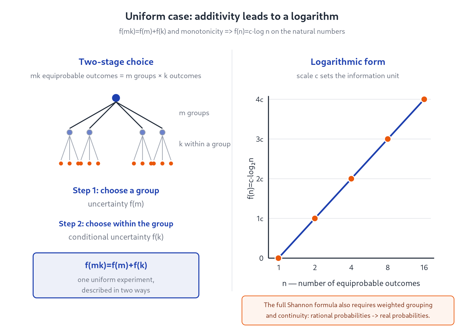
With base $2$, an event of probability $1/2$ has surprisal $1$ bit, and an event of probability $1/8$ has surprisal $3$ bits. Two independent fair coin flips produce four equiprobable sequences and $2$ bits: one bit for the first choice and one for the second. The logarithm is not decorative. It expresses exactly the requirement that independent stages add.

For a uniform source with $n$ outcomes, every outcome has probability $1/n$, so every outcome has surprisal

$-\log_2\frac1n=\log_2 n.$

This is already Hartley's answer: the number of equiprobable alternatives is measured logarithmically. A non-uniform source requires one additional step—average surprisal using the probabilities of the outcomes themselves:

$$H(P)=\mathbb E_{X\sim P}\!\left[-\log_2 P(X)\right] =-\sum_x P(x)\log_2P(x).$$

This is Shannon's formula, developed in detail in Module 2. Here it appears not as notation to memorize in advance, but as the answer to two successive requirements: rare outcomes should be more surprising, and independent stages should contribute additively.

Why this is immediately recognizable in ML

An autoregressive model factorizes a sequence probability into conditional probabilities:

$q(x_{1:T})=\prod_{t=1}^T q(x_t\mid x_{<t}).$

Taking a logarithm turns the product into a sum:

$$-\log_2 q(x_{1:T}) =\sum_{t=1}^T -\log_2 q(x_t\mid x_{<t}).$$

For one observed sequence, this quantity is its negative log-likelihood (NLL). Averaging such quantities over a dataset gives the model's empirical cross-entropy against the data. This is why NLL and cross-entropy are often used side by side in ML practice, even though one names the loss of an observation or a dataset and the other names an expectation or empirical average.

The token-level NLL contributions add to the loss of the whole sequence. The same sum gives the ideal code length when the predictive probabilities are fed to an entropy coder. A physical file includes coder overhead, and a complete system may also need to account for storing or transmitting the model itself, but the prediction–code-length connection is already exact.

Where the short derivation ends

Additivity gave us logarithmic surprisal and $\log n$ for a uniform source. It is not yet enough to single out Shannon's formula on every non-uniform distribution: Rényi entropies are also additive on independent products and also equal $\log n$ for the uniform distribution.

The full derivation needs a stronger idea. If a choice is made in two stages, total uncertainty should equal the uncertainty of the first stage plus the average conditional uncertainty of the second. This weighted grouping rule is the bridge from the uniform case to $-\sum p_i\log p_i$. Sections 1.9–1.10 build the bridge in full; on a first pass, it is enough to know why the bridge is necessary.

1.4. How the course is structured and how to read it

The main route and the second pass

Every module has a main ML route and explicitly marked mathematical deepenings. The main route starts with a recognizable problem, introduces the minimum mathematics needed, and returns to models, data, or training. A deepening preserves a complete proof, more general conditions, and counterexamples, but it is not an entrance exam.

The separation is already working in this module. To continue, it is enough to distinguish probability, surprisal, and meaning; understand the scope of the Shannon frame; and see the short logarithmic mechanism in §1.3. The full derivation of entropy is valuable, but it is better read as a second layer after entropy has become a familiar working object.

Terminology

The English version uses standard professional terminology directly. In the Russian version, an important English equivalent is given at first occurrence, while the explanatory prose remains predominantly Russian. Names of methods, APIs, and established abbreviations—softmax, logits, teacher forcing, ELBO, InfoNCE, RLHF, DPO, and PyTorch—retain their standard forms in both versions.

For the same reason, the Russian version of this module carries one extra reference note on the words выпуклая and вогнутая, whose everyday Russian meanings invite the opposite reading of convex and concave. English needs no such note, so the two versions of Module 1 differ by one section and their later section numbers are offset by one. Every other module is numbered identically in both languages.

The shape of a typical module

A module begins with a question: why do we need the new object at all? Then come the intuition, formal model, and key equation. A short proof remains in the main text when it exposes the mechanism; a long technical argument moves to a deepening. We then examine a classical example, a direct ML application, the boundary of the interpretation, and an exercise or computation that checks understanding.

The order matters. KL, mutual information, or MaxEnt can easily become a gallery of symbols. It is much more useful to see which engineering question produced the formula, what the formula guarantees, and which reasoning error it prevents.

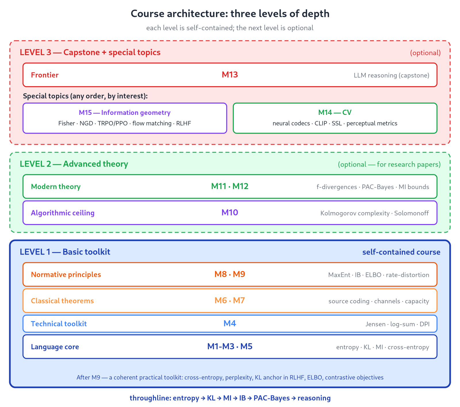
The pace is deliberately flexible. One module may take an evening or a week. The main M1–M9 route already forms a self-contained practical layer; M10–M13 add advanced theory and frontier topics; M14–M15 are optional specializations.

The required route through Module 1 ends here. Continue with Module 2. Skim §1.5 as a course map if useful; return to the literature and reference sections when needed; and open §§1.9–1.10 when you want the complete mathematical mechanism.

1.5. Course program: overview

The course is arranged as four concentric rings—from the core language of classical Shannon theory to its modern extensions in ML.

Language core (Modules 2–3 and 5). Entropy, cross-entropy, KL divergence, and mutual information are the fundamental measures on which everything else rests. Technical Module 4 is an insurance policy: Jensen's inequality and the associated toolkit, without which later modules become needlessly strained.

Classical Shannon theory (Modules 6–7). Source and channel coding theorems. Here the theory meets engineering reality: compression and communication. This is the historical root of the subject, and it is also where links to modern ML begin to flicker—the thesis that compression can test intelligence, context as a limited resource, attention as a possible channel analogy. These are perspectives and heuristics, not direct corollaries of Shannon's theorems.

Principles of inference (Modules 8–9). MaxEnt, IB, and rate–distortion. Here information theory becomes a normative framework for constructing systems. Softmax arises as the solution to an “expected score plus entropy regularization” problem; the optimum of KL-regularized RLHF has a Gibbs form relative to the reference policy; a VAE admits rate–distortion and information-bottleneck interpretations. Each claim requires an explicitly stated optimization problem—without one, attractive analogies become too strong.

Extensions (Modules 10–13). Algorithmic information theory; $f$-divergences and variational characterizations; information-theoretic generalization (PAC-Bayes and MI bounds); and a frontier module on reasoning in LLMs. These topics go beyond classical communication engineering and show how far information-theoretic language reaches in modern ML—sometimes as an exact theorem, sometimes as a research model.

Bonus modules (optional). Two additional modules extend the course sideways from the main path:

• Module 14—Information theory in computer vision. Neural image codecs as a continuation of Module 6 for continuous sources; links between diffusion models, estimation, score identities, and I–MMSE; contrastive, self-distillation, and masked-reconstruction methods in CV; perceptual losses and distributional metrics. Not all of these methods maximize mutual information, and LPIPS, SSIM, and FID are not information-theoretic divergences—the module separates direct theorems from useful interpretations.
• Module 15—Information geometry. Fisher information as a Riemannian metric on a statistical manifold, natural gradients, and the local quadratic approximation of KL by the Fisher matrix. KL itself is not a Riemannian distance. This module deepens Modules 3, 4, and 11. Target audience: ML engineers working in RL, normalizing flows, or delicate optimization regimes where ordinary gradient descent suffers from poorly conditioned parameterizations.

Three levels of depth. The course is deliberately designed so that you can stop after any of three levels and still have a coherent, self-contained picture:

• Level 1—the basic toolkit (M1–M9). Enough for a practicing ML engineer: entropy, KL/CE, MI, Shannon's source and channel coding theorems, MaxEnt, and IB/ELBO/rate–distortion. After M9, you understand the information-theoretic meaning of cross-entropy loss, perplexity, the KL anchor in RLHF, ELBO in VAEs, and MI interpretations of some contrastive objectives. This is the complete practical foundation.
• Level 2—advanced theory (M10–M12). Algorithmic information theory (Kolmogorov, Solomonoff, AIXI), $f$-divergences and variational characterizations, PAC-Bayes, and MI generalization bounds. This is the advanced theoretical layer above Level 1, intended for readers of current research and those planning to conduct it.
• Level 3—capstone and special topics (M13 + M14, M15). Reasoning in LLMs as a synthesis of the course (M13). Bonus Modules 14 (CV) and 15 (information geometry) deepen the material for specific audiences.

Concrete recommended paths are given in §1.7.

The detailed program and complete reading list are collected in the reference §§1.7–1.8. The references are grouped by role—backbone texts, proof references, specialist sources, and original papers—and are best consulted when a particular topic becomes interesting or difficult.

1.6. Literature: where to start

The course is not tied rigidly to a single textbook. Different sources play different roles.

Polyanskiy & Wu, Information Theory: From Coding to Learning (2025) is the modern backbone. The connection between information theory and learning is central from the first page, which matches the spirit of this course.

MacKay, Information Theory, Inference, and Learning Algorithms (2003) is the classic ML-oriented text. It is freely available from the author's site and remains exceptional for intuition and the Bayesian viewpoint.

Cover & Thomas, Elements of Information Theory is the reference for careful proofs when Polyanskiy–Wu or MacKay are terse.

Murphy, Probabilistic Machine Learning: An Introduction and Probabilistic Machine Learning: Advanced Topics provides the bridge between our modules and contemporary probabilistic ML more broadly.

Specialist references—Tsybakov for nonparametrics, Yamanishi for MDL, Jurafsky–Martin for NLP, the MIT VisionBook for CV, and Amari for information geometry—are listed in §1.8 together with original work by Shannon, Tishby, Hutter, and the Russian-language references. Do not try to read everything in advance; it is far more effective to consult a source when interest or difficulty arises.

1.7. Reference: detailed course program

This subsection gives a detailed description of every module. It is not part of the required first-pass route: return to it while progressing through the course to recall what comes next or why a topic is distributed across several modules.

Program

Module 1. Introduction. Information versus meaning—Shannon deliberately separated semantic questions from the engineering theory of communication, and that decision became both a fundamental strength of the theory and its natural limitation. The main route explains why an additive measure of surprisal must be logarithmic and connects that fact to NLL in autoregressive models. Optional §§1.9–1.10 give the complete axiomatic derivation, from the uniform source through weighted grouping and continuity to Shannon's formula.

Module 2. Entropy. $H(X)=\mathbb{E}[-\log p(X)]$ as expected surprisal. Properties: non-negativity, concavity, and the maximum at the uniform distribution. Joint and conditional entropy; the chain rule $H(X,Y)=H(X)+H(Y\mid X)$. Classical: fair and biased coins; Shannon's guessing experiment for English and his estimate on the order of $0.6$–$1.3$ bits per character under the particular experimental setup. ML/LLM: entropy of the output distribution as a measure of its spread—not the same as calibration or epistemic uncertainty; how post-training, decoding, and temperature alter entropy, without a universal claim that every instruction-tuned model must have lower entropy than its corresponding base model.

Module 3. Cross-entropy and KL divergence. The distinction between source entropy and the expected length of a code built from a different model. Definitions of $H(P,Q)$ and $D_{\mathrm{KL}}(P\|Q)$; the identity $H(P,Q)=H(P)+D_{\mathrm{KL}}(P\|Q)$; Gibbs' inequality. KL asymmetry and the familiar mode-covering/mode-seeking effects that arise under restricted approximation families—effects of typical optimization setups, not absolute properties of every algorithm. ML/LLM: empirical negative log-likelihood estimates cross-entropy; if CE is measured in bits, $\mathrm{PPL}=2^{\mathrm{CE}}$, if measured in nats, $\mathrm{PPL}=e^{\mathrm{CE}}$, and in general $\mathrm{PPL}=b^{\mathrm{CE}_b}$. The role of a reference policy and KL regularization in PPO-like RLHF and in the derivation of DPO.

Module 4. Jensen's inequality: a compact ML toolbox. The main route covers Jensen, equality conditions, the log-sum inequality, convexity of KL, two forms of ensembling, and the derivation of ELBO. It remains a technical module, but every formula is tied to a recognizable ML problem. Later subjects are no longer developed prematurely: sufficient statistics move to Module 8, IWAE to Module 9, Donsker–Varadhan and $f$-GAN to Module 11, and PAC-Bayes to Module 12.

Module 5. Mutual information. $I(X;Y)$ as an entropy difference, as the KL divergence between the joint distribution and the product of marginals, and as expected reduction in uncertainty. The Data Processing Inequality. MI detects any dependence in the sense that $I(X;Y)=0$ if and only if $X$ and $Y$ are independent in the standard setting, whereas zero correlation rules out only linear dependence. ML: InfoNCE as a contrastive objective and, under the appropriate sampling scheme, a lower bound on MI; the Information Bottleneck; MINE and the difficulty of estimating MI in high dimensions. Interpretations of attention as information exchange, or of residual connections through SDPI, will be labeled explicitly as research lenses rather than consequences of DPI.

Module 6. Source coding. Kraft's inequality and two levels of the source-coding theorem. For an optimal binary prefix code for one symbol from a finite alphabet, with entropy measured in bits, $H(X)\le L^*<H(X)+1$. For long blocks from a stationary ergodic source, average length per symbol can approach the entropy rate. Huffman coding, arithmetic coding, the AEP, and typical sets. ML/LLM: the operationally exact correspondence between probabilistic prediction and lossless compression through entropy coding, including finite coding overhead; the results of Delétang et al. as a striking demonstration, with the caveat that their published compression ratios do not include the storage cost of model parameters. Scaling laws may describe cross-entropy approaching some limit, but identifying that limit with the “true entropy of language” requires additional assumptions. Bits per character and bits per byte are useful tokenizer-independent units, but not the only legitimate ones.

Module 7. Channels and channel capacity. For a discrete memoryless channel, capacity is $C=\max_{p(x)}I(X;Y)$. The channel coding theorem, BSC, BEC, the Gaussian channel, and the Shannon–Hartley formula. ML/LLM: a context window, hidden states, and attention can be discussed in the language of limited information flow, but this is a modeling analogy: a transformer architecture does not become a discrete Shannon channel without an explicit specification of inputs, noise, constraints, and a transmission criterion.

Module 8. The maximum-entropy principle. Jaynes' principle: among distributions satisfying stated constraints, choose one of maximum entropy. Under linear expectation constraints, the solution—when it exists—has exponential form. This is connected to exponential families, but is not identical to the Pitman–Koopman–Darmois theorem: under regularity conditions, that theorem characterizes i.i.d. families admitting a sufficient statistic of fixed dimension. In regular exponential families, maximum likelihood produces moment matching when a finite interior solution exists. Softmax satisfies the exact variational formula, when $H(q)=-\sum_i q_i\ln q_i$ is measured in nats and $\tau>0$:

$\operatorname{softmax}(z/\tau)=\arg\max_{q\in\Delta}\left\{\mathbb{E}_{i\sim q}[z_i]+\tau H(q)\right\}.$

For unconstrained optimization over policies supported on the reference policy, the problem

$\max_\pi\;\mathbb{E}_{y\sim\pi(\cdot\mid x)}[r(x,y)]-\beta D_{\mathrm{KL}}\!\left(\pi(\cdot\mid x)\|\pi_{\mathrm{ref}}(\cdot\mid x)\right)$

has, for $\beta>0$ and a finite normalizing constant, the solution $\pi^*(y\mid x)\propto\pi_{\mathrm{ref}}(y\mid x)e^{r(x,y)/\beta}$. This is an exact statement about the specified optimization problem; its connection to Goodhart effects is a useful engineering interpretation, not a separate MaxEnt theorem.

Module 9. Information Bottleneck, ELBO, and rate–distortion. The IB principle, rate–distortion theory, and variational objectives. The VAE ELBO naturally decomposes into a distortion/reconstruction term and a rate/KL term; its relationship to variational IB is real but depends on which variables are designated as input, representation, and target. ML: self-supervised representation learning, quantization of weights and activations, and the debate over IB interpretations of neural-network training dynamics. Beyond the classical core: for $Y=\sqrt{\mathsf{snr}}X+N$, where $N\sim\mathcal N(0,1)$ is independent of $X$, $\mathbb E[X^2]<\infty$, and mutual information is measured in nats,

$\frac{d}{d\mathsf{snr}}I(X;Y)=\frac12\operatorname{mmse}(\mathsf{snr});$

when information is measured in bits, the right-hand side acquires an additional factor $1/\ln2$. I–MMSE, Tweedie/score identities, and denoising provide important bridges to diffusion models, but score matching does not follow from the I–MMSE identity alone.

Module 10. Algorithmic information theory. Kolmogorov complexity, the invariance theorem, and uncomputability; Solomonoff's universal lower-semicomputable semimeasure and its associated predictor; AIXI as an idealized, uncomputable agent. ML/LLM: MDL, Occam's razor, and a cautious analogy between a large language model and a computable approximation to universal prediction—an analogy, not an established theorem of Hutter about concrete LLMs. Landauer's principle, predictive information, and the free-energy principle can be discussed nearby, but FEP comes from variational inference and statistical physics rather than being a direct consequence of Kolmogorov complexity.

Module 11. $f$-divergences and variational characterizations. The class of $f$-divergences includes KL, total variation, $\chi^2$, squared Hellinger, and Jensen–Shannon divergence. Rényi divergence should be treated separately: at a fixed order it is related by a monotone logarithmic transformation to the corresponding Hellinger/power $f$-divergence, but it is not itself an $f$-divergence in general. Donsker–Varadhan for KL, the Gibbs variational principle, Pinsker's inequality, and other relations. ML: the original minimax GAN, with an optimal discriminator in the idealized setup, is connected to JS divergence; f-GAN extends the construction to $f$-divergences; MINE uses the DV representation.

Module 12. Information-theoretic generalization. PAC-Bayes and bounds through mutual information between the sample and the output of the learning algorithm. These bounds can be data- and algorithm-dependent and are therefore conceptually subtler than crude parameter counting, but for deep networks they are often difficult to compute or numerically vacuous. Why LLMs generalize well despite overparameterization remains an open research problem; MDL, flatness, and information-theoretic bounds offer different partial explanations, not a completed theory.

Module 13. Reasoning in LLMs through information theory (frontier). A capstone module in which channels, bottlenecks, compression, and algorithmic search are used as research models of reasoning. Chain-of-thought can be modeled as a sequential computational process with intermediate state, but it should not be identified without proof with “repeated uses of a channel,” nor should CoT depth be treated as a direct approximation to Solomonoff search. The frontier section includes Ton, Taufiq & Liu, “Understanding Chain-of-Thought in LLMs through Information Theory” (arXiv 2024; ICML 2025), and other recent work; claims here must be separated especially carefully into theorems, empirical findings, and hypotheses.

Bonus modules (optional)

Two additional modules extend the course away from its main path. They are written so that they may be skipped, taken out of numerical order, or selected according to interest. They depend on the core course M1–M13, but the core course does not depend on them.

Module 14. Information theory in computer vision (bonus). Neural image compression is directly connected to rate–distortion and learned entropy models. For generative modeling, I–MMSE, denoising, and score identities are useful. Representation-learning methods must be distinguished: SimCLR, MoCo, and CLIP use contrastive objectives; DINO is self-distillation without labels; MAE is masked reconstruction of pixels. They can be compared through information-theoretic lenses, but they cannot all be declared MI-maximization methods without an additional derivation. LPIPS is a learned perceptual feature distance, SSIM is a structural similarity index, and FID is the squared $2$-Wasserstein distance between Gaussian approximations to feature distributions, usually Inception features; none is an $f$-divergence or an “information-theoretic divergence” in the standard sense. MSE is appropriate for squared-error/PSNR objectives, although it often correlates poorly with human perceptual quality.

Module 15. Information geometry (bonus). Distributions as points on a statistical manifold, the Fisher information matrix $G(\theta)$ as a Riemannian metric, and the natural gradient

$\widetilde\nabla_\theta L=G(\theta)^{-1}\nabla_\theta L.$

This expression uses nonsingular $G$ in a regular parameterization; the singular case requires working on the identifiable space (§15.3).

KL is neither a metric nor a Riemannian distance, but for nearby parameters and under regularity conditions,

$D_{\mathrm{KL}}(p_\theta\|p_{\theta+d\theta})=\frac12d\theta^\top G(\theta)d\theta+o(\|d\theta\|^2).$

Regular exponential families have a dually flat structure with respect to a pair of dual affine connections; this does not mean that the Fisher–Rao metric has zero curvature in every sense. TRPO approximately solves a KL-constrained surrogate problem and is closely related to natural-gradient methods, but is not “the exact natural gradient.” PPO clipping is a practical heuristic and does not guarantee a strict trust region. K-FAC approximates Fisher/Gauss–Newton curvature under particular assumptions; Shampoo is a structured preconditioner in the full-matrix AdaGrad/second-order-inspired family, not simply another Fisher approximation.

Recommended paths through the course

The course is designed so that you can choose the depth that fits your goals and time. Each path below is self-contained: after completing it, you will have a coherent picture at that level.

Basic path—M1–M9 (approximately 30–40 hours). An information-theoretic toolkit for practical work. It covers the main constructions that repeatedly appear around cross-entropy loss, perplexity, KL regularization, ELBO, contrastive objectives, and rate–distortion. M9 is a natural stopping point with a complete, self-contained picture. This path suits ML engineers who want the mathematical foundations of everyday methods without yet moving deeply into research theory.

Full core course—M1–M13 (approximately 60–80 hours). Adds advanced theory to the basic path: M10 on algorithmic information theory, M11 on $f$-divergences and variational characterizations, M12 on PAC-Bayes and MI generalization bounds, and the capstone M13 on reasoning in LLMs. This path is intended for readers of current theoretical-ML research and those planning to do their own.

Full course with a CV focus—M1–M9 + M14 + the key parts of M11. The basic path plus the computer-vision bonus module: neural codecs, diffusion through I–MMSE, contrastive methods in CV, and perceptual losses. Sections 11.4–11.5 on f-GAN and MINE are required because they are used directly in M14. This path is for CV engineers who want information-theoretic foundations tailored to their domain.

Full course with a theoretical focus—M1–M13 + M15. The full core course plus the bonus module on information geometry. It suits ML engineers working in RL (natural policy gradients), normalizing flows, and delicate optimization—settings in which ordinary gradient descent encounters poorly conditioned parameterizations.

Notes. Bonus Modules 14 and 15 are not required for the main line of the course. They may be taken in either order after M13, or selected according to interest. If you want both, the order does not matter; they are independent.

1.8. Reference: complete annotated reading list

Materials

The course is not tied rigidly to a single textbook. Sources are grouped by the role they play.

Modern backbone: mathematical rigor with a contemporary presentation.

• Polyanskiy & Wu, Information Theory: From Coding to Learning (2025)—the primary modern reference for rigorous proofs and the connection between coding and learning.
• MacKay, Information Theory, Inference, and Learning Algorithms (2003)—a classic that develops information theory together with Bayesian inference and machine learning. It is freely available from the author's site and remains outstanding for intuition.

Classical proofs and reference material.

• Cover & Thomas, Elements of Information Theory, 2nd ed. (2006)—the canonical reference for careful proofs.
• Csiszár & Körner, Information Theory: Coding Theorems for Discrete Memoryless Systems—a deep treatment of the combinatorial side of the subject.

Probabilistic-ML companion.

• Murphy, Probabilistic Machine Learning: An Introduction and Probabilistic Machine Learning: Advanced Topics (2022, 2023)—the standard modern bridge from this course to probabilistic ML more broadly.

Specialist references.

• Tsybakov, Introduction to Nonparametric Estimation (2009)—for information-theoretic lower bounds using Fano, Le Cam, and Assouad.
• Yamanishi, Learning with the Minimum Description Length Principle (2023)—a deeper treatment of MDL.
• Jurafsky & Martin, Speech and Language Processing, 3rd ed., online manuscript (2026)—the NLP domain reference.

Practice and code.

• Zhang, Lipton, Li & Smola, Dive into Deep Learning—practical Python material for entropy, cross-entropy, and KL divergence.

Model quantization (for Module 9).

• Frantar et al., GPTQ (ICLR 2023); Lin et al., AWQ (MLSys 2024); Xiao et al., SmoothQuant (ICML 2023)—post-training quantization methods for LLM deployment. They illustrate the engineering trade-off among size, speed, and error, but are not direct consequences of the rate–distortion theorem.

Computer vision (for Module 14).

• Torralba, Isola & Freeman, Foundations of Computer Vision (MIT VisionBook, 2024)—the general modern CV background.
• Ballé, Laparra & Simoncelli, End-to-end Optimized Image Compression (2017), and Ballé et al., Variational Image Compression with a Scale Hyperprior (2018)—foundational neural-codec papers.
• Blau & Michaeli, Rethinking Lossy Compression: The Rate-Distortion-Perception Tradeoff (2019)—the theoretical foundation for §14.4.
• Mentzer et al., High-Fidelity Generative Image Compression (HiFiC, 2020)—a practical perceptual codec.
• Radford et al., Learning Transferable Visual Models From Natural Language Supervision (CLIP, 2021)—the basis of §14.5; an IB interpretation is possible but is not the paper's primary claim.
• Chen et al., A Simple Framework for Contrastive Learning (SimCLR); He et al., Momentum Contrast (MoCo); Grill et al., Bootstrap Your Own Latent (BYOL); Caron et al., Emerging Properties in Self-Supervised Vision Transformers (DINO); Oquab et al., DINOv2; He et al., Masked Autoencoders Are Scalable Vision Learners (MAE)—the main SSL families discussed in §14.6.

Information geometry, reinforcement learning, and generative flows (for Module 15).

• Amari, Information Geometry and Its Applications (Springer, 2016)—the root textbook reference for Module 15.
• Amari, Natural Gradient Works Efficiently in Learning (1998)—the foundational natural-gradient paper.
• Schulman et al., Trust Region Policy Optimization (2015) and Proximal Policy Optimization Algorithms (2017)—the basis of §15.5.
• Kakade, A Natural Policy Gradient (2001)—the transition from natural gradient to RL.
• Haarnoja et al., Soft Actor-Critic (2018)—maximum-entropy reinforcement learning.
• Martens & Grosse, Optimizing Neural Networks with Kronecker-factored Approximate Curvature (K-FAC, 2015); Gupta, Koren & Singer, Shampoo (2018); Anil et al., Scalable Second-Order Optimization for Deep Learning (2020)—structured preconditioning and curvature approximations.
• Lipman et al., Flow Matching for Generative Modeling; Liu et al., Flow Straight and Fast; Song et al., Score-Based Generative Modeling through Stochastic Differential Equations—the basis of §§15.6–15.7.
• Ouyang et al., Training Language Models to Follow Instructions with Human Feedback (InstructGPT); Rafailov et al., Direct Preference Optimization—the RLHF/DPO capstone.

Russian-language resources.

• Vereshchagin, Uspensky & Shen, Kolmogorov Complexity and Algorithmic Randomness (Russian edition, MCCME, 2013)—a fundamental treatment of algorithmic information theory.
• Vyugin, Mathematical Foundations of Machine Learning and Prediction (Russian edition, MCCME, 2022)—a modern book covering PAC-Bayes and online learning.
• Yandex School of Data Analysis handbook: Entropy and the Exponential Family—a useful Russian-language companion to Module 8.

Frontier reasoning.

• Ton, Taufiq & Liu, Understanding Chain-of-Thought in LLMs through Information Theory (ICML 2025)—an information-theoretic analysis of CoT steps.

Original papers worth reading in full.

• Shannon, A Mathematical Theory of Communication (1948)—one of the great scientific papers of the twentieth century and unexpectedly readable.
• Tishby, Pereira & Bialek, The Information Bottleneck Method (1999)—the foundation of Module 9.
• Belghazi et al., MINE: Mutual Information Neural Estimation (2018)—neural variational estimation of MI.
• Delétang et al., Language Modeling Is Compression (ICLR 2024)—the direct bridge between information theory and modern language models.
• Hutter, Universal Artificial Intelligence (2005)—the foundation of Module 10.
• Guo, Shamai & Verdú, Mutual Information and Minimum Mean-Square Error in Gaussian Channels (2005)—the I–MMSE identity and its diffusion connection.
• Amari, Natural Gradient Works Efficiently in Learning (1998)—the foundational NGD paper.

For intuition.

• MacKay's Cambridge lecture recordings.
• 3Blue1Brown's visual explanation of entropy through Wordle.

1.9. Optional mathematical deepening I: the uniform source

Second pass. No later module requires you to remember the details of this proof. Its purpose is to show that the logarithm was not guessed from an attractive formula; it is forced by consistency of multistage choice.

Let

$f(n):=H\!\left(\frac1n,\ldots,\frac1n\right)$

denote the uncertainty of a uniform choice among $n$ alternatives. We need two requirements.

Monotonicity. Increasing the number of equiprobable alternatives should not reduce uncertainty.

Consistency of a two-stage choice. Choosing one of $mk$ equiprobable outcomes can be described as choosing one of $m$ equiprobable groups and then one of $k$ elements inside the chosen group. Therefore

$f(mk)=f(m)+f(k).$

Now we can prove the precise result.

Theorem. If $f:\mathbb N\to\mathbb R$ is non-decreasing and

$f(mk)=f(m)+f(k)$

for all $m,k\ge1$, then there is a constant $c\ge0$ such that

$f(n)=c\ln n.$

Proof. Set $m=k=1$:

$f(1)=f(1)+f(1),$

so $f(1)=0$. Monotonicity then gives $f(n)\ge0$ for every $n\ge1$.

There is a small but important branch in the argument. The axioms allow the degenerate solution $f\equiv0$, corresponding to $c=0$. If the solution is non-degenerate, there is some $a\ge2$ with $f(a)>0$. Fix such an $a$.

The functional equation gives, by induction, for every integer $r\ge0$,

$f(u^r)=r f(u).$

Now fix any $n\ge2$. For each $r\ge1$, define

$s_r=\left\lfloor r\log_a n\right\rfloor.$

Then

$a^{s_r}\le n^r<a^{s_r+1}.$

Because $f$ is non-decreasing,

$f(a^{s_r})\le f(n^r)\le f(a^{s_r+1}).$

Using the power identity,

$s_r f(a)\le r f(n)\le(s_r+1)f(a).$

We may divide by $r f(a)$ because $r>0$ and $f(a)>0$:

$$\frac{s_r}{r} \le \frac{f(n)}{f(a)} \le \frac{s_r+1}{r}.\qquad (1)$$

The definition of $s_r$ also gives

$$\frac{s_r}{r} \le \log_a n < \frac{s_r+1}{r}.\qquad (2)$$

Both $f(n)/f(a)$ and $\log_a n$ lie in an interval of length $1/r$. Hence

$\left|\frac{f(n)}{f(a)}-\log_a n\right|\le\frac1r.$

The left-hand side does not depend on $r$, while the bound holds for every $r$. Letting $r\to\infty$ yields

$\frac{f(n)}{f(a)}=\log_a n.$

Therefore

$$f(n)=f(a)\log_a n =\frac{f(a)}{\ln a}\ln n =c\ln n.$$

In the non-degenerate case $c>0$; including $f\equiv0$ gives $c\ge0$. $\blacksquare$

What exactly have we proved?

We obtained the logarithmic form only for uniform distributions. Continuity was not used: the function is still defined on natural numbers. Extending the result to arbitrary probabilities requires weighted grouping, a substantively stronger requirement than mere additivity for independent sources.

1.10. Optional mathematical deepening II: from grouping to Shannon entropy

Second pass. This section completes the derivation. The central idea matters more than the technique: the uncertainty of a multistage choice should decompose like the expected cost of traversing a decision tree.

Consider a function $H(p_1,\ldots,p_k)$ on finite probability vectors. Relabeling outcomes changes nothing; zero-probability outcomes may be removed; and $H$ is continuous on the simplex.

The key requirement is weighted grouping. Suppose we first choose group $i$ with probability $p_i$, then choose outcome $j$ inside it with conditional probability $q_{j\mid i}$. Then

$$H\bigl(p_iq_{j\mid i}:i,j\bigr) =H(p_1,\ldots,p_m) +\sum_{i=1}^m p_i H(q_{1\mid i},\ldots,q_{k_i\mid i}).$$

This is the finite chain rule: uncertainty of the first stage plus average uncertainty of the second.

Step 1. Rational probabilities

Let $p_i=n_i/N$, where the $n_i$ are positive integers and $N=\sum_i n_i$. Imagine $N$ equiprobable micro-outcomes grouped into blocks of sizes $n_1,\ldots,n_k$. The same micro-outcome can be chosen in two ways.

Choosing directly among all $N$ outcomes costs $f(N)$. Choosing a group first and then an element within the group costs

$H(p_1,\ldots,p_k)+\sum_{i=1}^k p_i f(n_i).$

Weighted grouping makes the two descriptions equal:

$f(N)=H(p_1,\ldots,p_k)+\sum_i p_i f(n_i).$

Insert the result of §1.9, $f(n)=c\ln n$:

$$\begin{aligned} H(p_1,\ldots,p_k) &=c\ln N-c\sum_i p_i\ln n_i\\ &=-c\sum_i p_i\ln\frac{n_i}{N}\\ &=-c\sum_i p_i\ln p_i. \end{aligned}$$

Shannon's formula now holds for every distribution with rational probabilities.

Step 2. Arbitrary probabilities

Rational points are dense in the probability simplex. Continuity extends the formula to arbitrary real probabilities:

$H(p_1,\ldots,p_k)=-c\sum_i p_i\ln p_i,$

with the convention $0\ln0:=0$.

The axioms still allow the zero measure $H\equiv0$. A normalization both excludes it and chooses the unit. Requiring

$H\!\left(\frac12,\frac12\right)=1\ \text{bit}$

sets $c=1/\ln2$ and gives the familiar expression

$H(p_1,\ldots,p_k)=-\sum_i p_i\log_2p_i.$

Why independent-source additivity is not enough

It is easy to draw too strong a conclusion here. Rényi entropies

$$H_\alpha(P)=\frac{1}{1-\alpha}\log\sum_i p_i^\alpha, \qquad \alpha>0,\ \alpha\ne1,$$

are also additive for independent distributions and also equal $\log n$ on the uniform distribution. A logarithmic scale and product additivity therefore do not single out Shannon entropy. What singles it out is weighted grouping: the second-stage uncertainty is weighted by the probability of reaching each branch.

The counterexample worked out

It is worth seeing the counterexample concretely, because the qualitative claim above is easy to accept without noticing how sharp it is. Take Rényi entropy of order $2$:

$H_2(P)=-\log_2\sum_i p_i^2.$

It has the logarithmic value on a uniform source. For $U_n=(1/n,\ldots,1/n)$,

$\sum_{i=1}^n\left(\frac1n\right)^2=\frac1n,$

so

$H_2(U_n)=-\log_2\frac1n=\log_2n.$

It is additive on independent products. For independent $P=(p_i)$ and $Q=(q_j)$,

$$\begin{aligned} H_2(P\otimes Q) &=-\log_2\sum_{i,j}(p_iq_j)^2\\ &=-\log_2\left(\sum_i p_i^2\right) \left(\sum_j q_j^2\right)\\ &=H_2(P)+H_2(Q). \end{aligned}$$

And yet weighted grouping fails. Let

$P=\left(\frac12,\frac14,\frac14\right).$

Computed directly,

$H_2(P)=-\log_2\frac38=\log_2\frac83\approx1.415.$

Now describe the same choice in two stages: first the group $\{1\}$ or $\{2,3\}$ with probabilities $(1/2,1/2)$, then the outcome inside the selected group. The Shannon-style right-hand side would be

$$H_2\!\left(\frac12,\frac12\right) +\frac12H_2(1) +\frac12H_2\!\left(\frac12,\frac12\right) =1+0+\frac12=1.5.$$

The two numbers disagree: $1.415$ against $1.5$. So $H_2$ passes both weaker tests and fails the grouping identity, which is exactly why the derivation above needed the stronger axiom. Note also what this does not contradict: §§1.9–1.10 never claimed that a logarithmic scale and product additivity are sufficient. They are necessary consequences of the axioms, and $H_2$ shows they are not enough on their own.

The formula has now been derived rather than postulated or guessed. Multistage choice forces the logarithm in the uniform case, grouping transfers it to rational probabilities, continuity closes the real simplex, and normalization selects bits.