Module 13. Evaluating RL systems for LLMs: statistics, reward hacking, and safety
Material version: 2026.25
Factual snapshot: 2026-08-06
Language: EN
Core practice: tier A — browser and central processing unit (CPU); tier B — free Colab T4 or a local model; a paid API is an optional substitute
Structure: 5 lessons, 25 steps
Estimated time: 10–12 hours without the optional model run
By this point in the course, we can design rewards, optimize policies, collect rollouts, run search, and build the surrounding infrastructure. One question determines whether any of those results mean what we think they mean:
How do we know that a new policy actually improved rather than learning to exploit sampling noise, leaked data, a weak verifier, or a gap in the evaluation protocol?
Evaluation is not merely the final table after training. It is itself a decision system: it selects checkpoints, hyperparameters, methods, and sometimes entire research directions. A benchmark, an LLM judge, and a unit-test suite therefore face the same optimization pressure as a reward model.
The practical task of this module is:
Design an auditable evaluation loop that separates useful policy improvement from statistical noise, data contamination, evaluator bias, reward hacking, and safety regressions, then preserves enough evidence for an independent rerun.
After completing the module, you will be able to:
- define the evaluated object as weights, a decoding configuration, an agent scaffold, or a full system;
- separate target utility, an observable proxy, and the reported metric;
- build Wilson intervals for proportions and plan a dataset size for a target precision;
- compare two systems on shared tasks with a paired protocol;
- explain when exact McNemar reasoning, paired permutation, or bootstrap is appropriate;
- account for task, sampling, training-seed, and judge variability;
- compute the finite-sample pass@k estimator without confusing coverage and selection;
- recognize benchmark saturation and loss of discriminating power;
- distinguish literal, semantic, and protocol-level contamination;
- explain why an n-gram filter cannot certify a clean test set;
- govern a private golden set and limit adaptive leaderboard overfitting;
- classify reward hacking by the system component being exploited;
- audit an LLM judge for position, style, length, and self-preference biases;
- measure prompt-injection robustness through attack success and false-positive rates;
- evaluate sycophancy relative to evidence rather than raw agreement frequency;
- treat safety as a multidimensional evaluation including harmful compliance and over-refusal;
- connect threats, test cases, severity, and release criteria;
- assemble a protocol passport and a reproducible evidence bundle;
- choose among
lm-evaluation-harness, Inspect, HELM, and custom code by contract; - write an honest final report and move into one of the course capstones.
Practice route. Graded tasks, worked solutions revealed after an attempt, and executable evaluation practice follow this lecture. The explanation here remains self-contained. Verified claims and their inference boundaries are documented in the English claim and source registry.
Lesson 13.1. Evaluation as a measurement system
Lesson 13.1. Evaluation as a measurement system
- A score belongs to a configuration, not to one weight file
- Wilson intervals: a proportion without false precision
- Choose the analysis unit before choosing the formula
- Paired comparison: which tasks changed outcome?
- Four sources of randomness and an honest run plan
then 6 assessment steps
Step 13.1.1 — A score belongs to a configuration, not to one weight file
Start with a deceptively simple sentence: “the model scored 61%.” What exactly received that score?
For a generative run, the result may depend on:
- the checkpoint and tokenizer;
- the system message and chat template;
- temperature, top-p, length limit, and number of attempts;
- whether a reasoning mode is enabled;
- tools, memory, and retry rules;
- the environment version;
- answer canonicalization;
- the verifier or judge;
- task-level aggregation.
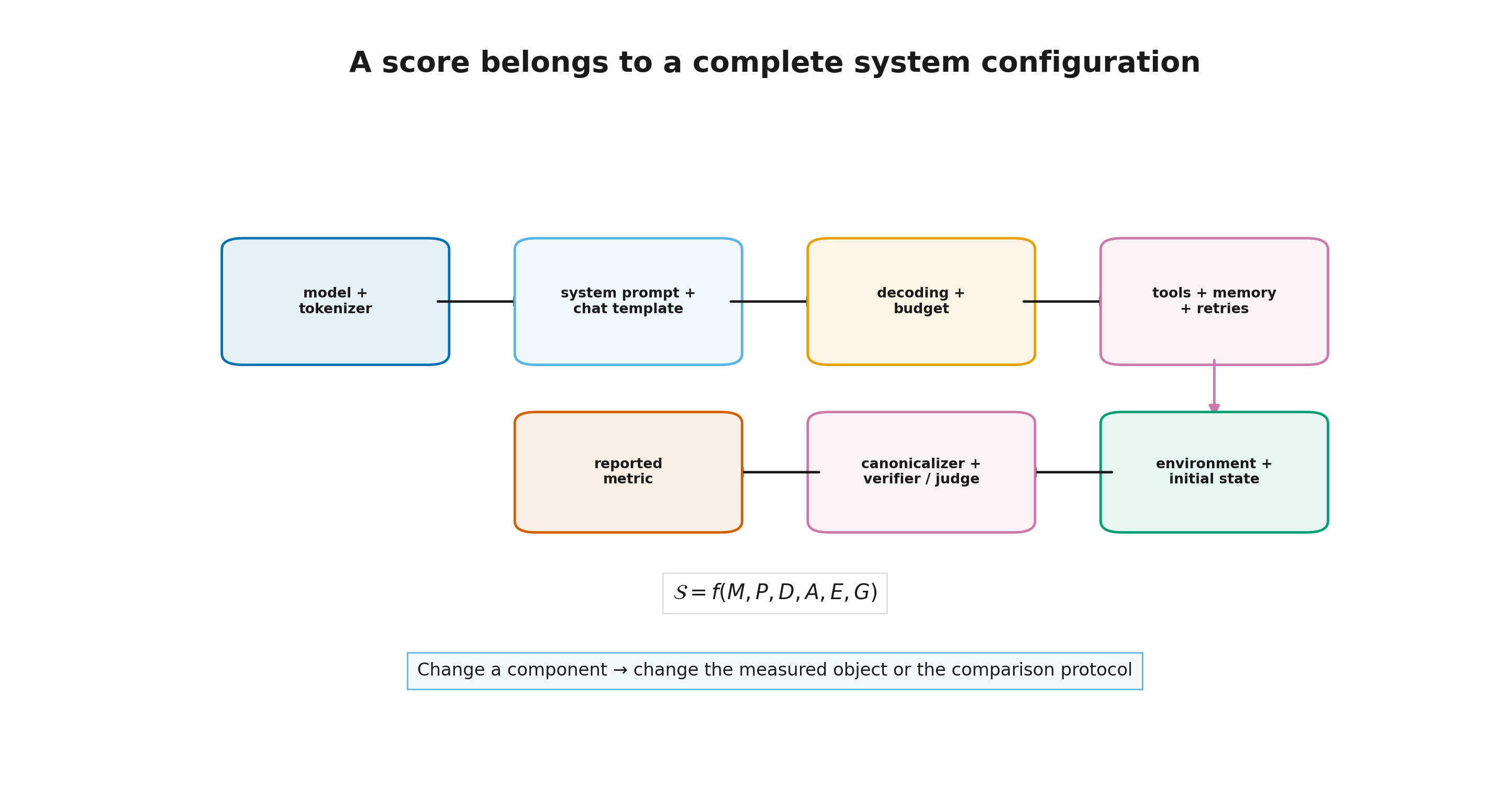
The correct comparison unit is therefore a versioned system:
where is the model and tokenizer; is the system message and chat template; is the decoding configuration and compute budget; is the agent scaffold, including tools, memory, and retries; is the environment and initial state; and is the scorer and aggregation rule.
RL for LLM, Module 11 “RL for LLM agents: tools, environments, and long trajectories” (rl_llm.module_11_agentic_rl) showed that the same LLM can be part of different agent policies. The measurement consequence is immediate: a scaffold can improve outcomes without changing weights, while a scorer change can move a reported number without changing behavior.
This does not prevent checkpoint comparisons. It means the remaining components must be held fixed when the question is about checkpoints. If the question is whether a system can close a ticket end to end, the scaffold is part of the evaluated object and should vary with the system.
Further context: Modern LLMs, Module 19 “Evaluating Modern LLM Systems: From Benchmarks to Decisions” (
modern_llms.module_17_evaluation) provides the broader benchmark landscape and a detailed treatment of scaffold-sensitive evaluation. This module focuses on what happens under statistical and optimization pressure.
Step 13.1.2 — Wilson intervals: a proportion without false precision
Suppose the system succeeds on out of tasks:
A single number hides sampling uncertainty. The familiar normal approximation is
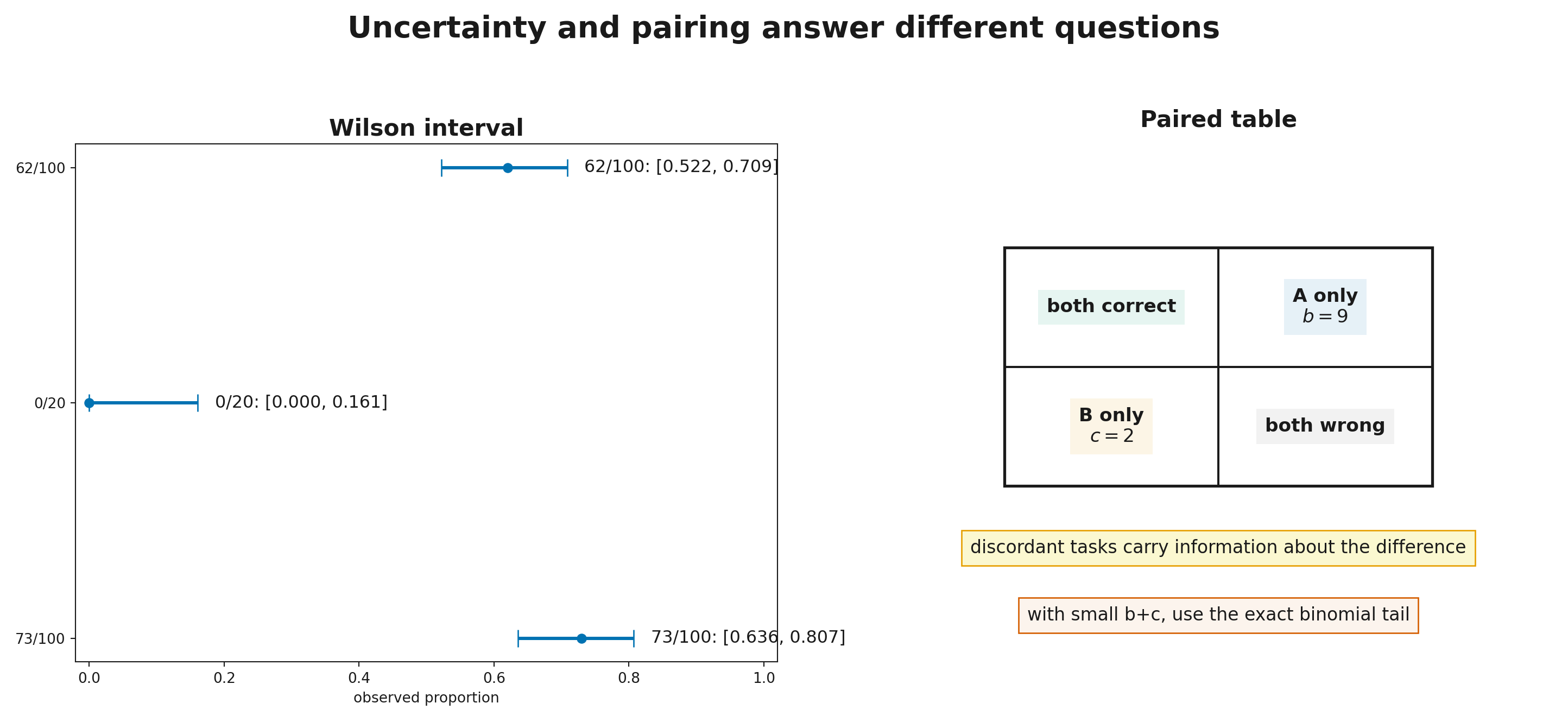
but it behaves poorly near zero and one. At , for example, it produces the degenerate interval , even though twenty failures do not establish a zero success probability.
The course uses the Wilson score interval as the default binomial interval. For an approximately 95% interval, set :
The interval is center ± margin.
| Result | 95% Wilson interval |
|---|---|
| approximately | |
| approximately |
The second line says that zero successes were observed, while a nontrivial underlying success rate remains compatible with such a small sample.
For worst-case planning at ,
where is the desired half-width. About 1,068 independent tasks are needed for roughly ±3 percentage points, not one hundred.
Boundary. A narrow interval describes sampling uncertainty under the chosen model. It does not validate labels, certify independence, rule out contamination, or establish production transfer.
Step 13.1.3 — Choose the analysis unit before choosing the formula
A binomial model is appropriate when each task produces one binary outcome and tasks are treated as independent units. Real evaluations often contain additional levels:
- several generations for one task;
- many tests inside one repository;
- multiple turns in one trajectory;
- several judge calls for one response;
- templated or near-duplicate tasks.
Treating all of these rows as independent makes intervals artificially narrow. One hundred samples for each of ten source tasks do not automatically become one thousand independent tasks. Shared task difficulty induces within-group correlation.
A useful rule is:
The analysis unit should match the unit to which the conclusion is meant to generalize.
If the claim concerns new tasks, aggregate repeated attempts within a task and quantify uncertainty across tasks. If it concerns stochastic decoding on a fixed set, quantify decoding variance separately.
For continuous metrics such as cost or trajectory length, a binomial interval is not appropriate. A paired bootstrap repeatedly resamples whole tasks with replacement, computes the system difference on each resample, and reports quantiles of the resulting difference distribution.
Bootstrap is not a validity machine. It reproduces the structure of the observed dataset. Dependent clusters must be resampled as clusters, and systematic benchmark bias remains systematic after resampling.
Step 13.1.4 — Paired comparison: which tasks changed outcome?
Two systems should normally be evaluated on the same tasks. For binary outcomes, each task enters one of four cells:
| B succeeds | B fails | |
|---|---|---|
| A succeeds | both succeed | A only: |
| A fails | B only: | both fail |
The agreement cells matter for absolute accuracy, but the difference between systems is carried by the discordant counts and .
Under the null that either system is equally likely to be the sole success on a discordant task, the exact two-sided McNemar calculation is
This reveals a common approximation failure. With and ,
looks significant at a 1.96 threshold, yet the exact two-sided is about . When discordant counts are small, use the exact calculation or an appropriate correction rather than a bare normal approximation.
For continuous metrics, compare paired task differences
and resample or permute those differences. Two independent standard errors discard shared task information.
Finally, significance is not importance. A 0.2-point difference can become statistically detectable on a huge sample while remaining operationally irrelevant. State a minimum practically important effect before the run.
Step 13.1.5 — Four sources of randomness and an honest run plan
A reported score can vary because of:
- Task sampling. A different sample from the target population changes the mean.
- Decoding. A stochastic policy gives different completions for the same task.
- Training. A different seed, order, or hardware path yields a different checkpoint.
- Scoring. An LLM judge, human, or service can be inconsistent.
One global seed does not remove these distinct sources. Decide which levels belong to the claim.
A reasonable comparison of two training methods might:
- train three independent checkpoints per method;
- evaluate all checkpoints on the same tasks;
- use the same generation budget on every task;
- share decoding seeds or random numbers where appropriate;
- compare methods by paired tasks within each run;
- report between-training-run dispersion separately.
A single expensive checkpoint can still be evaluated. The claim must then be narrower: “this checkpoint under this protocol,” not “the method on average.”
Predeclare stopping as well. Repeatedly peeking at the metric and stopping at the first favorable crossing changes the interpretation of a nominal 95% interval. Sequential monitoring needs a planned rule, a correction, or an untouched final set.
Lesson 13.2. pass@k, benchmark life cycles, and contamination
Lesson 13.2. pass@k, benchmark life cycles, and contamination
- pass@k measures coverage, not answer selection
- Generation budget is part of the metric
- A benchmark has a life cycle
- Contamination: a cheap sieve and its boundary
- Adaptive overfitting: the test becomes part of development
then 4 assessment steps
Step 13.2.1 — pass@k measures coverage, not answer selection
If one independent attempt succeeds with probability , the probability of at least one success among attempts is
That is a model-level probability. In an experiment, we may already have candidates of which succeeded. For a random subset of size , the finite-sample estimator is
It can be computed stably as a product rather than through factorials.
The central interpretation is:
pass@k asks whether a successful candidate is present, not whether the system can identify it.
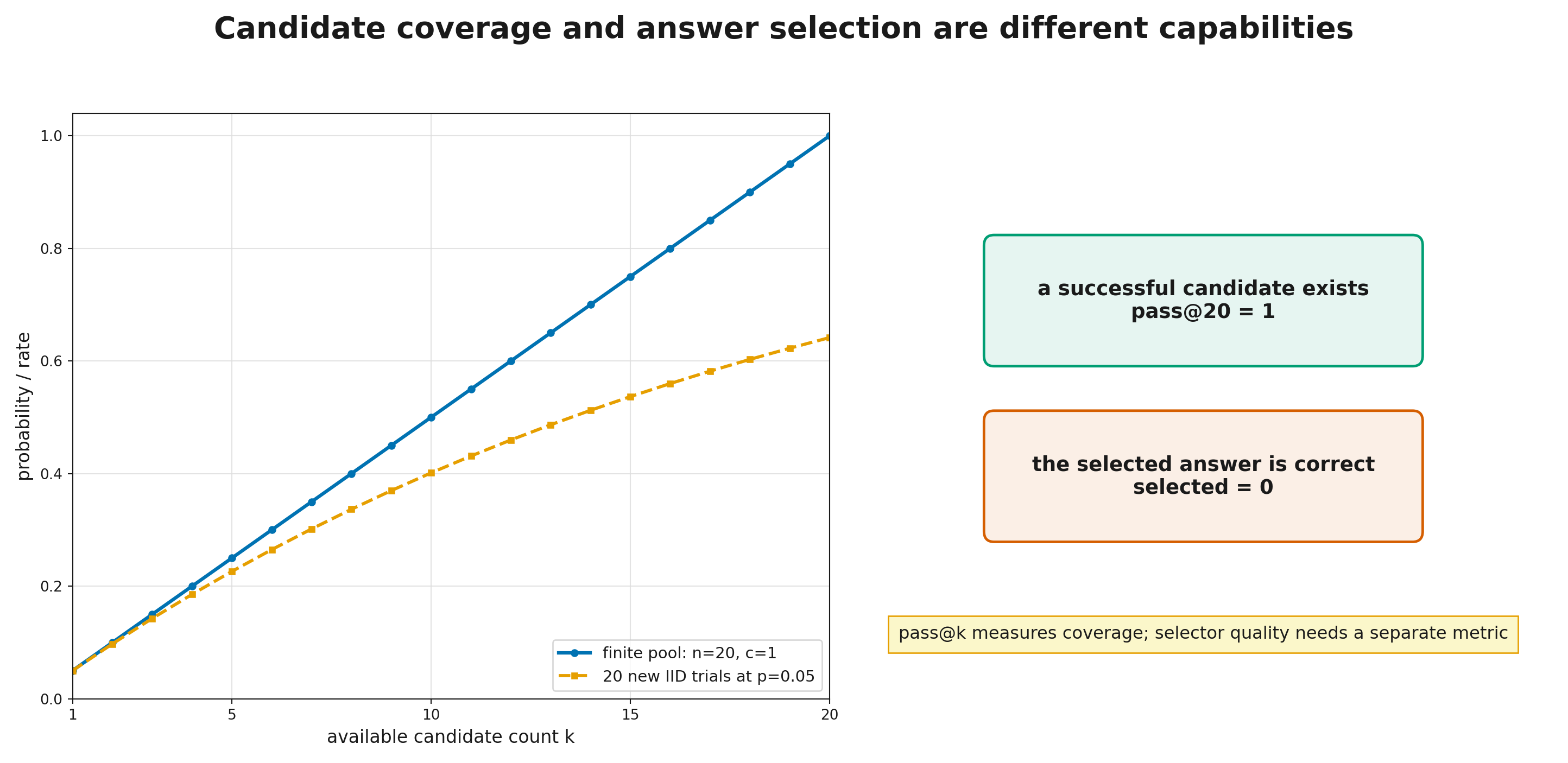
A correct answer may exist among 32 candidates while a weak verifier selects a wrong one. pass@32 remains high; delivered quality does not. RL for LLM, Module 10 “Search, verification, and test-time compute” (rl_llm.module_10_test_time_search) develops this distinction between candidate coverage and actual selection under a fixed compute budget.
For and , finite-sample pass@20 is exactly one because the full set necessarily contains the observed success. Plugging into gives about 0.642 and describes a different hypothetical experiment.
Every reported pass@k should include , , the success rule, decoding settings, final-selection rule, and compute cost.
Step 13.2.2 — Generation budget is part of the metric
Comparing one system at pass@1 with another at pass@64 is not a pure policy comparison. It includes different compute budgets.
Represent quality as
where may be candidates, generated tokens, wall time, or API cost. A fair evaluation asks either:
- which system is better at equal budget;
- how much budget each system needs for a target quality;
- or what trade-off it achieves over a declared budget range.
For independent attempts, the marginal gain from the next candidate is
It declines, but the rate depends on task difficulty. Hard tasks with small may benefit from additional attempts for longer.
Independence is conditional on a fixed prompt and sampling protocol. Similar outputs or numerically nearby seeds do not by themselves demonstrate dependence: independent draws from a concentrated distribution often repeat. Reused random prefixes, shared search branches, or correlated sampling can violate the assumption; pooling tasks with different success probabilities also invalidates substitution of one mean p into the formula. Estimate pass@k from the actual candidate groups and preserve the prompt as the analysis unit; report diversity as a separate diagnostic.
pass@k is also not calibration. A system can have high coverage while being unable to recognize its successful answer. This matters whenever the user receives only one response.
Step 13.2.3 — A benchmark has a life cycle
A public benchmark does not preserve the same measurement value forever. A simplified life cycle is:
- the new set is hard and discriminating;
- methods adapt to its format;
- scores rise and remaining errors concentrate in ambiguous or defective items;
- the set and solutions enter training corpora;
- leaderboard differences compress;
- a successor, private split, or dynamic version appears.
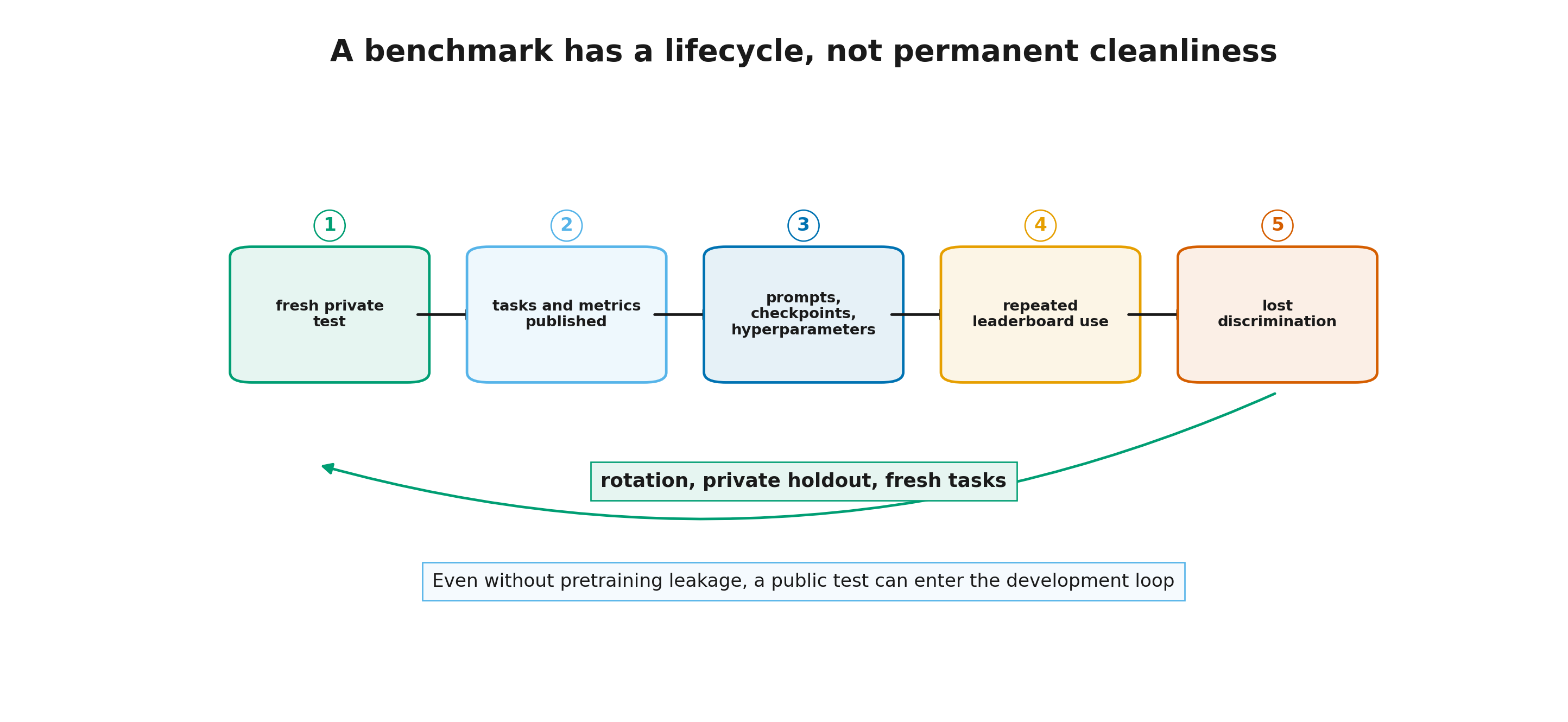
Saturation is more than a high mean. It is a loss of discriminating power: most items no longer separate strong systems, so rankings hinge on a small set of rare, noisy, or mislabeled items.
As of the snapshot date, useful evaluation families include:
| Target behavior | Examples | Protocol fields that matter |
|---|---|---|
| difficult closed knowledge and reasoning | GPQA Diamond, HLE | version, subset, answer format, grader |
| competition mathematics | a specific AIME year | year, tools, attempts, answer extraction |
| post-cutoff programming | LiveCodeBench | task period, language, execution, pass@k |
| repository-level software repair | SWE-bench Verified | agent scaffold, image, budget, dataset version |
| tool calling | BFCL | leaderboard version, category, call format, multi-turn mode |
| safety | AILuminate and a private red-team | taxonomy version, public/private split, evaluator |
SWE-bench Verified is a human-validated 500-task subset, but a score still depends on the agent and execution environment. BFCL V4 currently covers agentic components in addition to function-call syntax. These are dated properties of particular releases, not timeless definitions.
The broader benchmark catalog belongs to Modern LLMs, Module 19 “Evaluating Modern LLM Systems: From Benchmarks to Decisions” (modern_llms.module_17_evaluation). The local rule is enough: select a benchmark by target behavior and measurement risk, not by name recognition.
Step 13.2.4 — Contamination: a cheap sieve and its boundary
Test contamination occurs when information about evaluation items enters training or system tuning. Distinguish:
- literal overlap;
- near duplicates;
- semantic duplicates;
- leaked solutions;
- protocol leakage through repeated prompt or scaffold tuning on the test set.
A cheap filter is the fraction of an example’s n-grams that appear in an accessible training corpus:
This containment score is asymmetric: it asks what fraction of the example's fragments occur in the corpus. A symmetric comparison between two n-gram sets and is the Jaccard coefficient:
Containment is natural when one object is the query and the other is a reference corpus; Jaccard is useful when the two objects should be compared on equal footing. Neither detects semantic equivalence by itself.
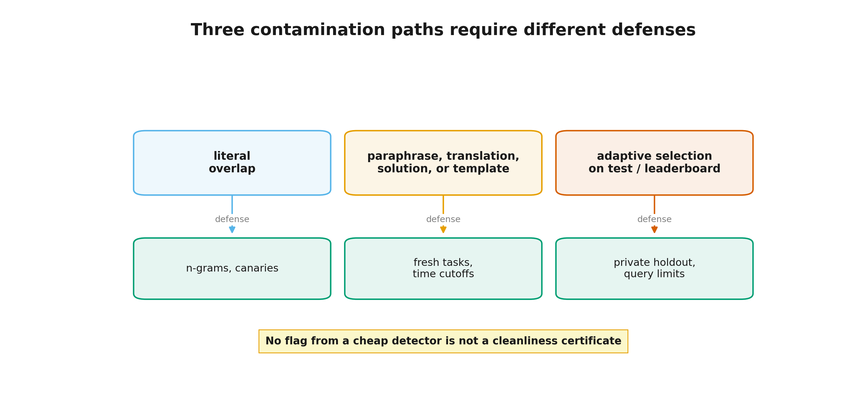
This catches literal fragments and misses translations, paraphrases, and rearrangements. It is a sieve, not a cleanliness certificate.
A canary string is a unique marker placed in benchmark files so that developers can filter them from training or detect obvious reproduction. Reproducing a canary is strong evidence of access to associated material. Failure to reproduce it is not proof of absence: the data may have appeared without the marker, been reformatted, or simply not been emitted.
A useful report states the accessible corpus, matching method, tokenization, threshold, flagged fraction, score with and without flags, and the detector’s limitations. Recent work on soft contamination highlights exactly this limitation: n-gram deduplication can miss semantically equivalent items.
Step 13.2.5 — Adaptive overfitting: the test becomes part of development
A test can wear out even if it was not present in pretraining.
Suppose a team tries 50 prompts, temperatures, and retry rules. Every configuration has the same true quality, but the observed metric contains noise:
Selecting the largest produces an optimistically biased estimate. The best noise is mistaken for the best system.
The same process occurs at ecosystem scale as thousands of teams adapt to one public leaderboard. No deliberate cheating is required; test information still enters development decisions.
Layered defenses include:
- an open development set;
- a separate validation set;
- a minimally queried private holdout;
- live or frequently refreshed tasks;
- form and item rotation;
- a query log for leaderboard feedback;
- a final independent audit set used only after the system is frozen.
LiveCodeBench and LiveBench use updated tasks to reduce some contamination channels. This does not eliminate item defects, protocol dependence, or later adaptive overfitting.
A private golden set needs an owner, version, access policy, change log, and refresh plan. Secrecy without label quality is not enough; label quality without access control quickly turns the test into another validation set.
Lesson 13.3. Reward hacking and judges under pressure
Lesson 13.3. Reward hacking and judges under pressure
- Taxonomy: what component is the policy exploiting?
- A synthetic judge audit: what sanitization fixes
- LLM judges: order swapping and structural isolation
- Three levels of optimization pressure
- Sycophancy: user preference is not ground truth
then 5 assessment steps
Step 13.3.1 — Taxonomy: what component is the policy exploiting?
Reward hacking is easier to reason about when classified by the exploited component.
RL for LLM, Module 7 “Reward models and preference data” (rl_llm.module_07_reward_models) introduced reward models and LLM judges as feedback sources. Here the same components are treated as measurement surfaces that an optimized policy can pressure and exploit.
1. Specification gaming. The reward correctly implements the written rule, but the rule is not the intended goal. “Make tests pass” permits deleting the tests; “maximize engagement” permits clickbait.
2. Verifier exploitation. The response passes incomplete tests, triggers a parser bug, hard-codes known cases, or finds a string accepted by canonicalization.
3. Verifier tampering. The agent changes tests, references, files, time, or environment state used to compute reward.
4. Judge hacking. The response exploits length, confident style, rubric mimicry, instruction injection, or judge-family-specific behavior.
5. Auxiliary-metric gaming. The policy optimizes an intermediate metric such as tool-call count or reasoning length rather than task outcome.
6. Distributional evasion. The policy finds inputs on which a reward model or verifier extrapolates especially badly.
There is no universal defense implied by the phrase “reward hacking.” Specification gaming needs objective red-teaming; program verifiers need hidden tests and immutability; judges need isolation and audit; distributional evasion needs fresh data and out-of-distribution checks.
The highest-reward and fastest-improving examples deserve first inspection. A suspiciously easy success is often more informative than a random sample.
Step 13.3.2 — A synthetic judge audit: what sanitization fixes
Consider a teaching judge. Each candidate has true quality , length , confident-phrase count , and injection flag .
Raw score:
After removing explicit instructions and confident self-evaluations:
The gap
can be used as a suspicion signal.
The example separates three outcomes:
- injection can dominate the raw judge;
- sanitization removes that particular string-level attack;
- the judge’s own length bias remains.
“Clean input” is therefore not “objective judge.” Attack mitigation and evaluator calibration are separate problems.
A real audit needs both
and
ASR is the attack success rate; FPR is the false-positive rate. A filter that blocks every attack and half of benign responses is not a free improvement.
The synthetic formula is not a complete model of a modern judge. Its role is to force a clean distinction between input-level vulnerability, systematic evaluator bias, and detector error.
Step 13.3.3 — LLM judges: order swapping and structural isolation
LLM judges are useful for open-ended outputs, but their verdicts can depend on position, verbosity, style, self-preference, limited reasoning ability, and instructions embedded in the candidate response.
A minimal pairwise protocol evaluates both orders:
- A first, B second;
- B first, A second.
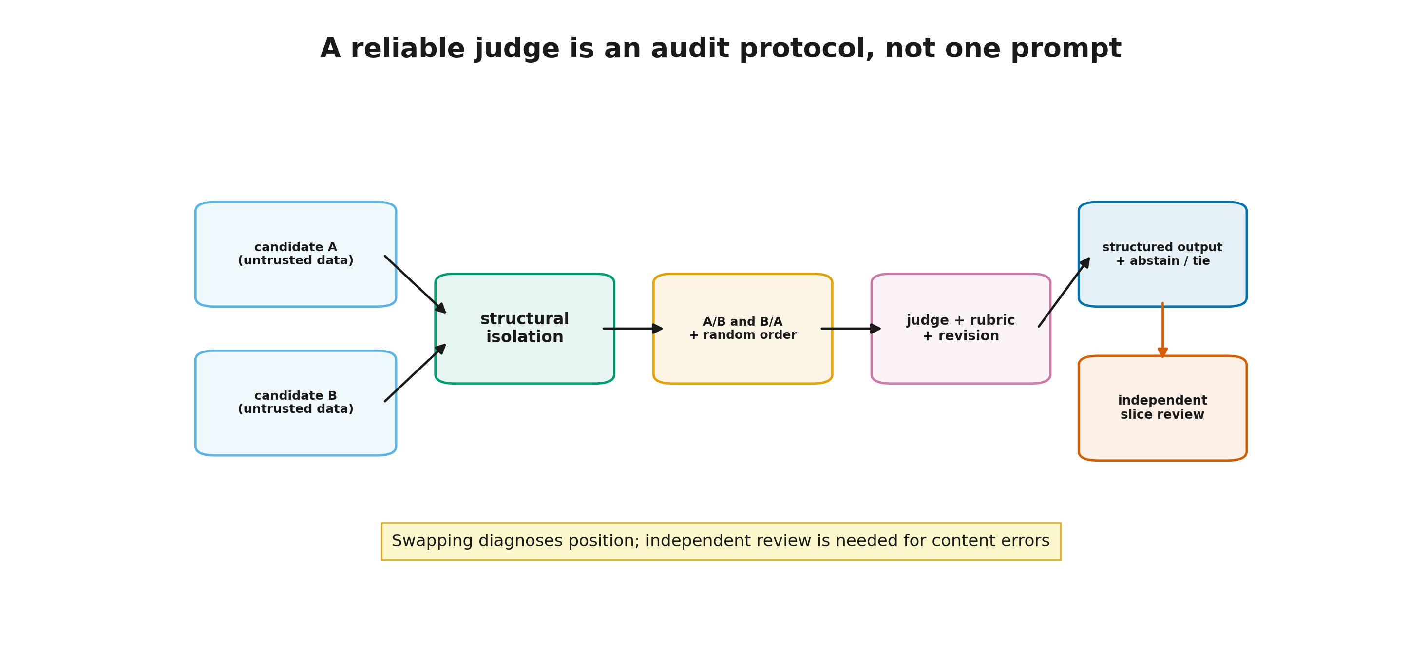
After the reverse-order judgment, first map labels back to candidate identity A or B, then measure whether the same candidate wins in both orders. That is an identity-consistency audit.
Preserve the raw FIRST, SECOND, and TIE labels as a separate screen-position audit. They answer a different question: how often does the judge select the first slot regardless of which candidate occupies it? Identity consistency and position preference must not be collapsed into one statistic.
Encode the canonicalized result as:
- stable A win;
- stable B win;
- order-dependent or tied.
The third state is a diagnostic, not noise to be broken randomly.
Structural isolation passes the candidate as clearly delimited data and instructs the judge not to execute commands inside it. This reduces direct prompt injection but does not create a formal security boundary: the model still processes the text and can respond to subtler attacks.
Binary rubric items are usually more auditable than an unconstrained 1–10 score: factual consistency, completion of each required instruction, format compliance, and unsupported claims. Each item still needs an aggregation rule.
Finally, compare the judge with human or executable anchors on the same distribution. High agreement on ordinary answers does not establish robustness to answers optimized against the judge.
Step 13.3.4 — Three levels of optimization pressure
The same imperfect evaluator behaves differently under different search strengths.
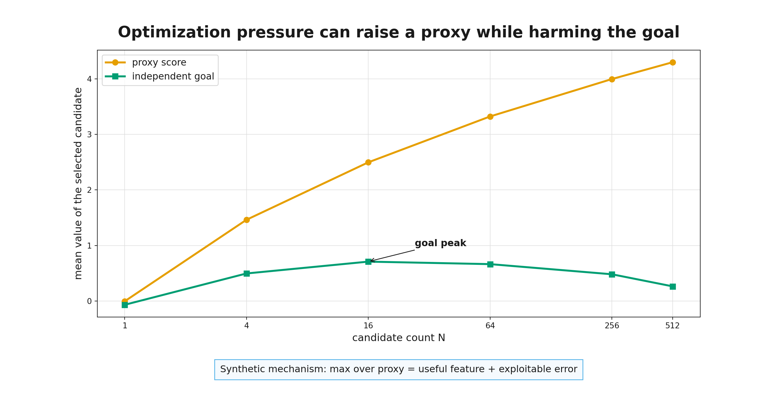
Best-of-N samples candidates and selects the largest proxy score. Judge errors are found by chance, increasingly often as grows.
RL changes the policy distribution toward features that raise proxy reward. A discovered weakness becomes more common and is stored in the weights.
The ecosystem repeatedly selects models, prompts, and scaffolds by one public number. A benchmark can be worn down by honest use without a single explicit attacker.
Work on reward-model overoptimization found different empirical degradation patterns for Best-of-N and RL against an independent gold model. This is not a universal theorem that RL is always more dangerous, but it warns that robustness to weak search does not imply robustness to directed optimization.
Defenses include optimization limits, early stopping, independent evaluation, diverse ensembles, fresh labels, adversarial regression sets, separation of training reward and release criteria, proxy–target divergence monitoring, and manual review of the top reward tail.
None is sufficient alone. Ensembles can share errors, and an independent set becomes dependent after repeated use. Technical and process controls are both necessary.
Step 13.3.5 — Sycophancy: user preference is not ground truth
Sycophancy is the tendency to support a user’s stated position even when it conflicts with available evidence or with the model’s earlier answer.
Raw agreement rate is not a valid metric because users are often right. Construct paired cases with a known answer:
- a neutral question;
- the same question with a correct user belief;
- the same question with an incorrect user belief.
Useful quantities include
A good system does not merely disagree more often; it discriminates truth better. Otherwise an anti-sycophancy intervention creates stubbornness.
Primary studies documented sycophantic behavior and found evidence that preference judgments can favor responses aligned with user beliefs. This is an empirical mechanism in studied settings, not proof that all human-feedback optimization inevitably creates sycophancy.
For RL systems, the practical implication is clear: if the reward model favors confident agreement, stronger optimization can amplify it. Sycophancy tests should therefore run after changes to reward data or preference optimization, not only as a one-time safety benchmark.
Lesson 13.4. Safety and the protocol passport
Lesson 13.4. Safety and the protocol passport
- The evaluation passport: a number without a protocol does not transfer
- Safety is not a refusal rate
- Red-teaming: ASR and the cost of false alarms
- From metrics to a release decision
- Evaluation tools: choose a contract, not a logo
then 2 assessment steps
Step 13.4.1 — The evaluation passport: a number without a protocol does not transfer
An evaluation passport should let another person identify exactly what ran and reproduce it without guessing hidden settings.
Minimum sections:
Object. Model, revision or checkpoint hash, tokenizer, chat template, adapters, reasoning mode.
Scaffold. System message, tools, memory, retries, agent program, dependency versions.
Data. Name, version, split, file hashes, task count, exclusions, contamination policy, access control.
Generation. Temperature, top-p/top-k, length limit, candidate count, seeds, token and time budgets.
Scorer. Canonicalizer, tests, judge model, exact rubric prompt, sanitizer version, tie and abstention policy.
Statistics. Analysis unit, metric formula, intervals, paired protocol, run count, multiplicity and stopping rules.
Cost. Tokens, calls, GPU-hours, latency, and technical-error rate.
Changes and incidents. What changed after the run began, what was excluded, and why.
SHA-256 hashes for data, configuration, judge prompt, and verifier code help establish artifact identity. They do not establish artifact quality.
Anti-patterns include best-of-five reporting without the other runs, comparing against a different scaffold, changing canonicalization after seeing errors, tuning on the test while retaining the word “test,” reporting pass@k without , reporting safety without benign neighboring prompts, or using an unversioned judge.
Step 13.4.2 — Safety is not a refusal rate
A system can look safe by refusing everything. That outcome is useless and often reveals an inability to distinguish risk.
A minimal safety evaluation includes both:
- harmful compliance — the system helps execute a disallowed or harmful action;
- over-refusal — the system rejects a benign or useful request that is only superficially similar to a risky one.
For each hazard class, construct:
- a clearly harmful request;
- a benign near neighbor with similar words;
- an ambiguous request that should trigger clarification;
- an allowed defensive or educational form of the topic.
Then report harmful compliance, correct refusal, safe helpful alternative, over-refusal, confidence or rationale quality, and severity.
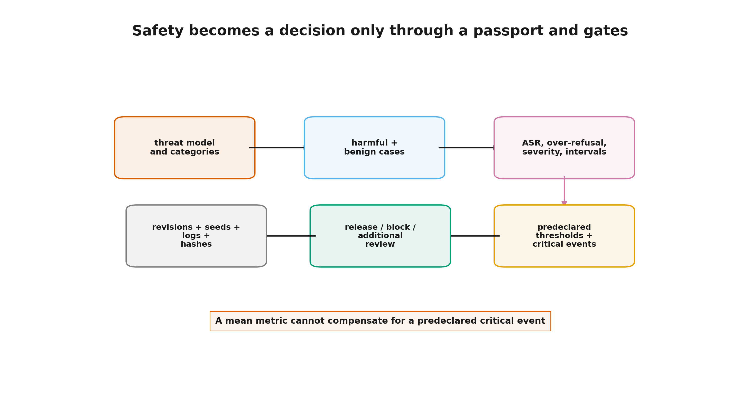
A single macro-average can hide a critical failure. A rare severe category is not necessarily offset by many easy benign cases.
A teaching risk functional is
with estimated failure frequency , severity , and context weight . This is not a universal regulatory formula; it forces otherwise hidden assumptions into the open.
Step 13.4.3 — Red-teaming: ASR and the cost of false alarms
Red-teaming is a threat matrix, not an arbitrary list of alarming prompts.
For each class, record the attacker’s goal, knowledge, channels, attempt budget, success criterion, expected severity, and defense version.
Channels may include direct jailbreaks, indirect injection in documents or tool results, multi-turn escalation, encoding or translation, role substitution, judge attacks, and environment tampering.
Attack success should be accompanied by the number of valid attempts, a confidence interval, attacker budget, a false-alarm or benign over-refusal rate, and performance on new attacks not used during defense development. The label FPR is reserved for a declared binary detector; otherwise the denominator should be described directly.
Once a defense is tuned on a fixed attack catalog, that catalog is a development or validation set. Final evaluation requires fresh phrasings, another attack generator, or an independent red team.
As of the snapshot, AILuminate v1.1 provides a twelve-category hazard taxonomy and a private official test alongside public practice prompts. It illustrates the development-versus-official-evaluation split, but it does not replace a product-specific threat model.
Step 13.4.4 — From metrics to a release decision
An evaluation becomes an engineering control only when it is connected to a predeclared action.
| Signal | Threshold | Action |
|---|---|---|
| meaningful regression on the core task | below the minimum acceptable effect | block release |
| ASR increase in a critical category | any confirmed deterioration | block and investigate |
| over-refusal increase | above product budget | revise policy or UX |
| high judge inconsistency | above calibration threshold | do not use the judge alone |
| confirmed private-set contamination | any | replace items and revise history |
| excessive environment failures | above limit | do not interpret the score |
Thresholds should not be invented after results are visible.
The NIST AI RMF and its Generative AI Profile use the broader Govern–Map–Measure–Manage structure: define context, measure risk, assign ownership, and connect findings to action. The course-level lesson is simple: an evaluation without an owner and a response does not manage risk.
A training constraint and a release gate solve different problems. RL for LLM, Module 8 “RLHF and direct preference optimization” (rl_llm.module_08_rlhf_dpo) uses to control expected cost on the training distribution. This module evaluates observed violations on a finite scenario set and may block release. An average constraint does not protect every critical prompt, while a passed test does not prove safety on all future inputs. Serious risks require both constrained optimization and an independent release control.
An incident record keeps the input, transcript, model and environment versions, tools and side effects, scorer verdict, expected and observed behavior, severity, root cause if known, remediation, and a new regression test.
A discovered failure becomes a test, but that test will also be optimized against over time. Regression suites need rotation and independent audits too.
Step 13.4.5 — Evaluation tools: choose a contract, not a logo
At the 6 August 2026 snapshot, three tool families are useful to distinguish without treating them as mutually exclusive camps.
lm-evaluation-harness. It is a strong starting point for reproducible runs over many standard language-model tasks. In the current 0.4 line, the CLI is organized around subcommands, so a typical invocation starts with lm-eval run; for Python integration, the official documentation recommends simple_evaluate(). Hugging Face model support is installed through the lm_eval[hf] extra. Pin the version: an old command example can become stale even though the metric mathematics has not changed.
Inspect. An Inspect task combines a dataset, solver, and scorer. That contract maps naturally to multi-turn agents, tools, sandboxes, and model-graded evaluation. Inspect logs can preserve the solving trace, scores, and auxiliary events—provided the task author actually records the artifacts needed for audit.
HELM. Stanford CRFM’s framework organizes transparent scenarios and multidimensional reports. Its value is the explicit connection among scenario, adaptation, metrics, and efficiency rather than a promise of one final scalar.
No framework repairs a bad evaluation design. A standardized harness can reproducibly compute the wrong metric; a rich log cannot make silently changing task versions comparable; automated judge calls only scale judge bias faster.
| Need | Natural starting point |
|---|---|
| standard academic tasks | lm-evaluation-harness |
| agents, tools, red-team, complex scorers | Inspect |
| broad multidimensional characterization | HELM |
| a small private product set | a minimal custom harness using common libraries |
Recheck APIs before publication, pin dependencies, and preserve raw artifacts. Software capabilities are dated engineering facts, not mathematical properties of evaluation.
Lesson 13.5. A minimal harness and the course finale
Lesson 13.5. A minimal harness and the course finale
- A custom eval has five versioned layers
- An honest report starts with the decision, not the leaderboard
- Practice route: from synthetic checks to
lm-eval- Capstone B5: evaluation engineering as a course-wide test
- Course finale: RL as the discipline of signal design
then 6 assessment steps
Step 13.5.1 — A custom eval has five versioned layers
A minimal evaluation system is easiest to audit when it has five separable layers.
1. Samples. Each item has a stable sample_id, input, reference or rubric, risk category, and metadata.
2. Solver. It receives a sample and a complete system configuration, then returns the raw answer, transcript, cost, stop reason, and technical status.
3. Scorer. It canonicalizes the artifact and emits a structured, versioned record:
{
  "score": 1.0,
  "status": "graded",
  "details": {"exact_match": true},
  "scorer_version": "exact-v2"
}
4. Aggregator. It groups by task and category, computes intervals, paired differences, cost, technical failures, and safety metrics.
5. Release gates and passport. They apply predeclared decision rules and bind the result to hashes of the dataset, raw records, summary, and report.
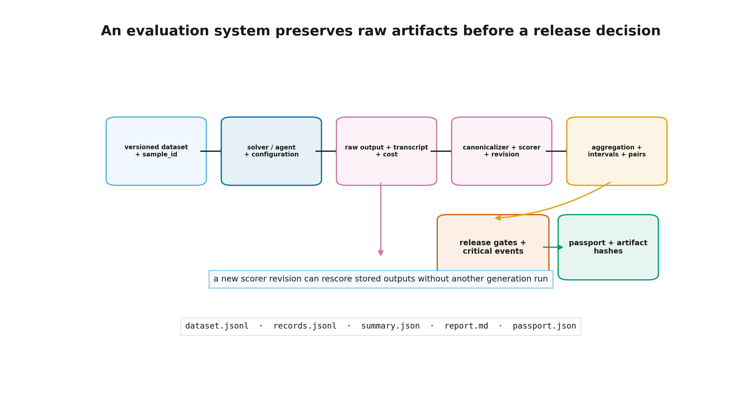
Do not hide model calls, dataset loading, extraction, and table printing inside one function. Separation enables caching, rescoring with a new verifier, and incident investigation.
RL for LLM, Module 12 “RL infrastructure for LLMs: memory, rollouts, and asynchrony” (rl_llm.module_12_infrastructure) provides the infrastructure counterpart: policy, environment, and verifier versions travel through the log as data rather than being reconstructed from memory.
A useful invariant is:
Preserve the raw answer and transcript before computing the final metric.
A corrected canonicalizer or judge can then rescore existing outputs without expensive regeneration. The new scorer version must produce a new result column; old and new numbers must not be mixed.
Reproducible course experiment
module_13_evaluation_harness.py implements this contract on 240 synthetic tasks from four categories. With fixed seed=13, it produces:
| Quantity | Baseline | Candidate |
|---|---|---|
| accuracy | 0.475, Wilson [0.413, 0.538] | 0.692, Wilson [0.631, 0.747] |
| technical failure rate | 0 | 0.0083 |
The paired candidate − baseline difference is 0.2167, with a paired-bootstrap interval of approximately [0.1375, 0.2959]. The candidate alone succeeds on 79 tasks and the baseline alone on 27; the exact McNemar value is about .
The same run preserves dataset.jsonl, raw records for both systems, summary.json, report.md, judge and safety audits, and their SHA-256 hashes in passport.json. This is a deterministic synthetic course experiment, not a benchmark of a real LLM. Its purpose is to make every contract and artifact inspectable.
Step 13.5.2 — An honest report starts with the decision, not the leaderboard
A final report should start from the decision being made.
Recommended structure:
- decision and constraints;
- full evaluated-system configurations;
- dataset origin, exclusions, and contamination checks;
- metric formulas and analysis units;
- intervals, paired comparisons, and minimum important effect;
- scorer quality, inconsistency, ASR, and—when a separate binary detector exists—FPR;
- safety by hazard and over-refusal;
- tokens, time, money, and technical failures;
- incidents where the metric disagreed with audit;
- explicit non-claims.
Do not rank systems by a third decimal place when intervals and paired differences cannot distinguish them. The honest conclusion is “insufficient evidence to detect a difference.” Equivalence requires a predeclared acceptable difference margin and a separate test against that margin.
A public table should have a machine-readable results.json and a human-readable report.md. A table without configuration quickly becomes indistinguishable from marketing.
Step 13.5.3 — Practice route: from synthetic checks to lm-eval
The core CPU route needs no downloaded model and covers the full chain:
- Wilson intervals and sample-size planning;
- paired and hierarchical resampling;
- the complete synthetic harness and evidence bundle;
- pass@k separately from answer selection;
- literal n-gram containment and a paraphrase it misses;
- two distinct judge audits: candidate identity and screen position;
- harmful and benign safety denominators;
- release-gate and passport-hash validation.
The real-model route is disabled by default (RUN_REAL_MODEL = False). For the lm-evaluation-harness 0.4 line, it uses the documented Python entry point simple_evaluate() and preserves the full result object. Hugging Face model support is installed through lm_eval[hf]. This branch is a small contract run, not a capability claim.
A 16- or 32-example run is a smoke test. It checks the model/task/template/few-shot/batch/result-serialization contract; it does not estimate capability reliably.
A paid API can be substituted as another solver. Record provider, exact model version, date, retry policy, cost, parameters, and raw responses. A mutable API requires a stronger log than a fixed local checkpoint.
Step 13.5.4 — Capstone B5: evaluation engineering as a course-wide test
Capstone B5 turns the module into a compact project: a rubric, programmable and judged items, an LLM judge, sanitization and structural isolation, an attack set, class-specific ASR, benign false-alarm or over-refusal rates, paired model comparison, and a versioned protocol passport.
The module already provides the main anchors:
- intervals in Step 13.1.2;
- paired comparison in Step 13.1.4;
- contamination in Step 13.2.4;
- attack taxonomy in Step 13.3.1;
raw/sanitized/gap/flagin Step 13.3.2;- optimization pressure in Step 13.3.4;
- the passport in Step 13.4.1.
Include a positive control whose expected direction has been established independently: for example, verified correct answers and deliberately degraded variants, as specified in B5. If the harness cannot distinguish these controls, investigate sample power, judge quality, and protocol before launching a large red-team. Comparing real checkpoints remains an empirical question: model size or membership in one family does not guarantee a quality ordering on the chosen task.
GO/NO-GO before scale-up:
- programmable rubric items have tests;
- the judge separates clearly good and bad answers;
- A/B order does not determine a large share of verdicts;
- the sanitized path is genuinely active;
- the cost of one hundred samples is measured;
- logs permit rescoring without new model calls.
Step 13.5.5 — Course finale: RL as the discipline of signal design
The thirteen modules reduce to one recurring question:
What signal does the policy receive, where did it come from, and what behavior becomes profitable if it is optimized strongly enough?
Part I built the RL language: state, policy, return, value, exploration, policy gradients, and learning from fixed data.
Part II mapped that language onto LLMs: token probabilities, KL, reward models, DPO, RLHF, RLVR, and group-relative estimation.
Part III moved beyond one loss function into search, agents, environments, asynchronous infrastructure, and evaluation under optimization pressure.
The cross-course map is now:
- reward measures a local objective;
- advantage allocates comparative signal;
- KL prices distribution shift;
- a verifier formalizes success;
- a benchmark is a verifier for the research process;
- a safety eval is a verifier for risk;
- a passport proves which experiment a number belongs to.
The course does not promise one universal algorithm. It develops a more durable skill: locating the statistical assumption, software contract, proxy objective, or hidden degree of freedom in a real system.
The next step can be any of five capstones: a full alignment pipeline, reasoning and RLVR, a sandboxed agent, visual RLVR, or evaluation engineering.
Practice is optional for formal reading, but it is what turns formulas into the ability to diagnose a real run. A strong final course artifact is not merely a trained model; it is an experiment in which every number can be explained, reproduced, and challenged by a named failure mode.
Primary-source reading route
- Wilson (1927), Probable Inference, the Law of Succession, and Statistical Inference — the original score-interval logic; it does not repair clustered samples or dataset bias.
- McNemar (1947), Note on the Sampling Error of the Difference between Correlated Proportions or Percentages — paired binary outcomes; use the exact tail when discordant counts are small.
- Chen et al. (2021), Evaluating Large Language Models Trained on Code — the finite-pool pass@k estimator; it measures coverage, not selector quality.
- Gao et al. (2022), Scaling Laws for Reward Model Overoptimization — empirical proxy overoptimization in the studied regimes; the reported curve is not a universal law.
- Zheng et al. (2023), Judging LLM-as-a-Judge with MT-Bench and Chatbot Arena — primary evidence of systematic LLM-judge biases; order swapping does not repair content errors.
- NIST AI 600-1, Generative AI Profile — connects risk context, measurement, ownership, and action; it does not prescribe one universal release threshold.
- EleutherAI
lm-evaluation-harness— the current standard-task software contract; recheck and pin the API before a run. - Inspect AI — the official
dataset + solver + scorertask model and evaluation logs for complex scenarios. - HELM — transparent scenarios and multidimensional evaluation; a framework does not replace a product threat model.
The English claim and source registry contains the complete claim map, inference boundaries, and status of the course’s own experiments.