Module 9. RLVR and GRPO: verifiable rewards, group-relative estimates, and stability
Material version: 2026.21
Factual snapshot: 2026-08-05
Language: EN
Core practice: level A — browser and central processing unit (CPU); level B — free Colab T4 with Low-Rank Adaptation (LoRA)
Structure: 5 lessons, 25 steps
Estimated time: 10–13 hours, excluding optional model training
Module 8 “RLHF and direct preference optimization” (rl_llm.module_08_rlhf_dpo) optimized a policy from a fixed preference dataset. We now let the policy create its own data: for each prompt it produces several responses, a checking procedure assigns rewards, and the next training update changes the distribution of future responses.
This regime is called reinforcement learning with verifiable rewards (RLVR). Group Relative Policy Optimization (GRPO) is often used for it, but the two names are not synonyms:
- RLVR describes the feedback source: a program, formal system, test suite, or environment can check the outcome;
- GRPO describes one way to estimate relative advantages and update a policy without a learned critic.
The practical problem of this module is:
Build a reproducible RLVR loop in which the reward actually checks the intended property and the chosen GRPO variant does not hide normalization bias, policy mismatch, or loss of diversity.
After completing the module, you will be able to:
- distinguish RLVR from GRPO, PPO, direct preference optimization, and inference-time search;
- explain the roles of current, old, and reference policies in a group update;
- derive group-relative advantages and the canonical clipped GRPO objective;
- explain why “critic-free” does not mean “baseline-free”;
- design a verifier and distinguish false-positive from false-negative rewards;
- compute the probability of an informative group and the cost of dynamic resampling;
- compare original GRPO, Dr. GRPO, DAPO, and GSPO by the exact unit of normalization and importance correction;
- diagnose entropy loss, length drift, truncation, and generation–training mismatch;
- discuss the “elicitation versus discovery” question without overstating pass@k evidence;
- run deterministic CPU exercises and prepare an optional experiment with a roughly 0.6-billion-parameter model.
Dated claims, primary sources, and explicit boundaries are recorded in Module_9_Sources.md. The practical route has its own English notebook, the executable practice.
Practice route. Graded tasks, worked solutions revealed after an attempt, and executable practice follow the lecture. The explanation remains self-contained.
Lesson 9.1. RLVR as a feedback contract
Lesson 9.1. RLVR as a feedback contract
- What makes a reward verifiable
- DeepSeek-R1-Zero as a historical case, not a universal recipe
- A verifier is a stack, not a single Boolean
- A numerical verifier: useful core, explicit limits
- When does a group carry a learning signal?
then 5 assessment steps
Step 9.1.1 — What makes a reward verifiable
An RL reward may come from a human, a learned model, an environment, or a physical measurement. RLVR identifies a narrower regime: there is a reproducible procedure that checks a response or trajectory.
Examples include:
- comparing a number or symbolic expression with a canonicalized reference;
- running code inside a sandbox against tests;
- checking a proof with a trusted formal kernel;
- evaluating a tool call by the resulting environment state;
- scoring a game or simulator trajectory under explicit rules.
Verifiable does not mean binary. A reward can be real-valued, multi-component, or partially graded. The essential requirements are that a fixed checker returns the same result for the same input and that the criterion is close enough to the property we actually want to improve.
The loop is
Here is a prompt, are responses sampled by the old policy, are checker outputs, and are relative estimates within the group.
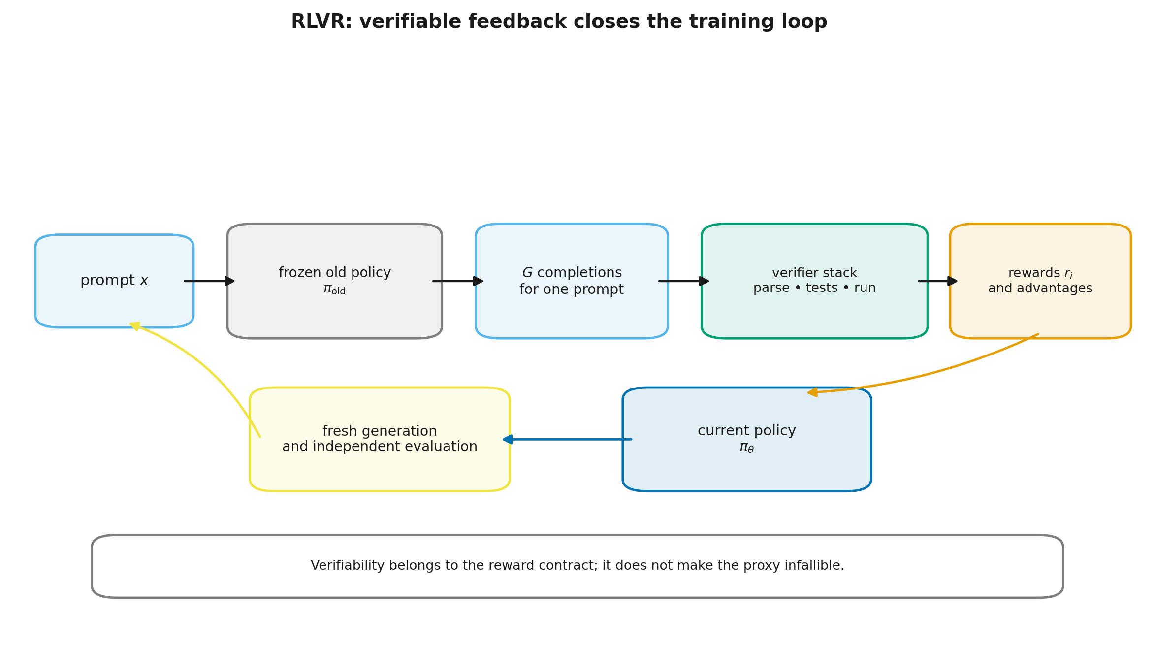
Boundary. Best-of-N with the same checker remains inference-time search when model parameters do not change. DPO remains fixed-data preference optimization when no fresh responses are collected inside the stage. RLVR begins when a verifiable outcome enters a policy update.
Step 9.1.2 — DeepSeek-R1-Zero as a historical case, not a universal recipe
The DeepSeek-R1 technical report presents DeepSeek-R1-Zero as an RL stage started directly from DeepSeek-V3-Base, without a preceding supervised stage containing labeled reasoning traces. The authors report that, during training, responses became longer and more often included intermediate checking, backtracking, and alternative approaches.
The report also documents serious limitations: poor readability, language mixing, and a narrow concentration on formally verifiable tasks. Final DeepSeek-R1 therefore used a multi-stage pipeline with cold-start data, further supervised fine-tuning, rejection-sampled data, and later RL stages. The historical lesson comes from both parts: the pure run shows that a verifiable signal can strongly reshape the response distribution, while the final pipeline shows that this stage alone is not a complete recipe for a generally useful model.
The R1-Zero reward is described through two rule-based components:
Mathematics used final-answer checking, code used compilation and tests, and a separate term encouraged the required response structure.
The compact GRPO formula displayed in the report includes a KL term with coefficient and a full-response probability ratio. The report does not, however, provide a machine-complete run passport from which every reference-policy schedule, rollout-reuse detail, and estimator choice can be reconstructed. The careful statement is therefore: the reported objective allows KL regularization; the actual coefficient and remaining engineering details belong to the versioned implementation or run configuration. “R1-Zero was definitionally GRPO with no KL whatsoever” and “every RLVR system should copy the R1 configuration” both go beyond the available evidence.
Epistemic status: pipeline design, reward types, and observed behavior are claims from the model authors’ technical report. They demonstrate one successful large-scale process, not that the absence of preliminary SFT, the same reward, or the same hyperparameters is optimal for another model or task distribution.
Step 9.1.3 — A verifier is a stack, not a single Boolean
“Reward equals correctness” hides a sequence of decisions:
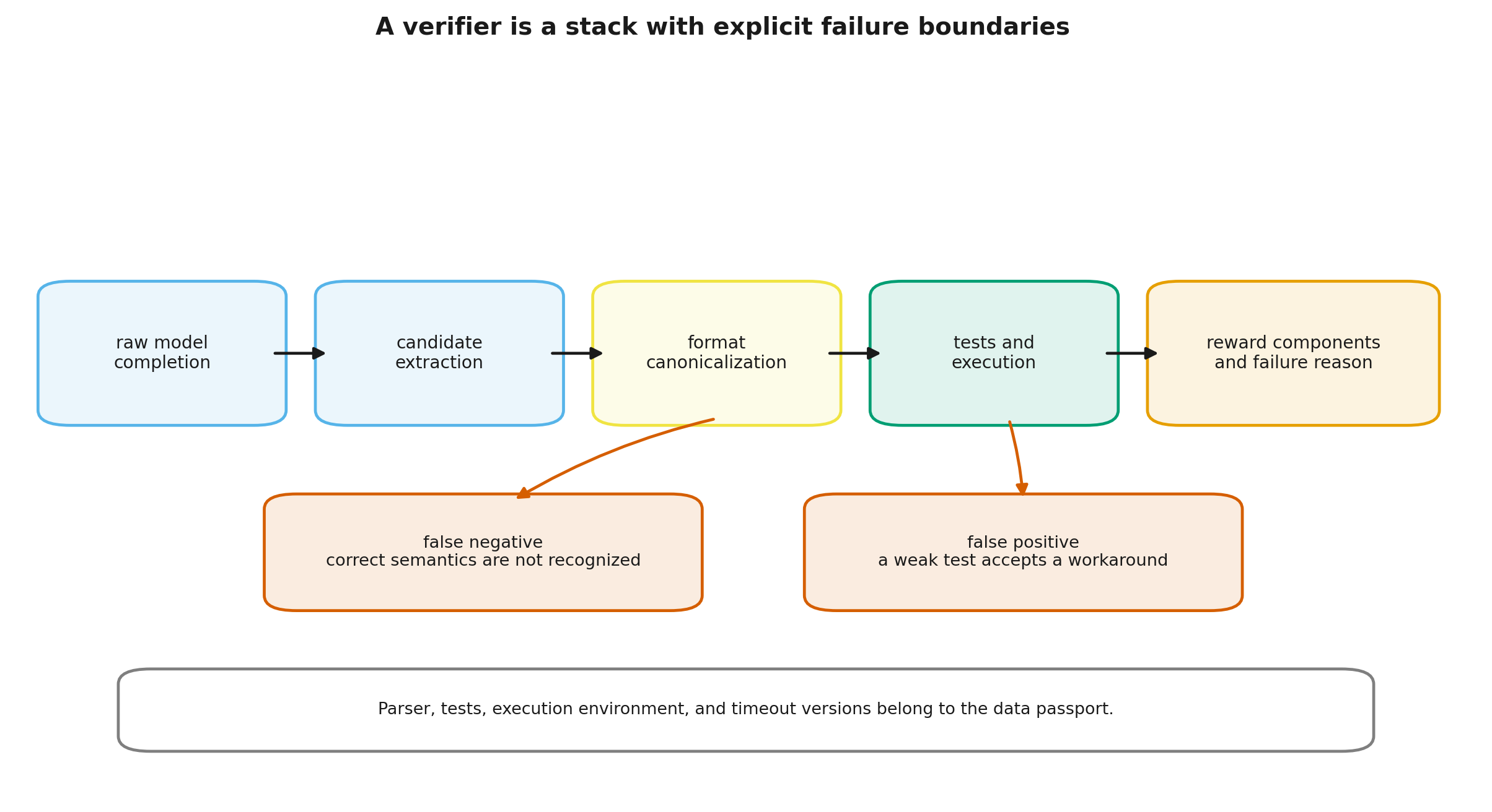
A numerical task must specify where the answer appears, how fractions are interpreted, whether rounding is accepted, and how multiple final answers are handled. Code adds language version, dependencies, time and memory limits, network and file-system access, randomness, and hidden tests.
Two errors have different consequences:
- false-positive reward: an incorrect response passes, giving the policy a direct incentive to exploit the checker;
- false-negative reward: a correct response fails, suppressing a useful trajectory.
False positives are especially dangerous under repeated optimization because a rare loophole can become the dominant strategy. False negatives make the signal sparser and reduce the effective number of successes.
A minimum checker passport records:
- parser and reference-answer versions;
- canonicalization rules;
- accepted formats;
- execution restrictions;
- positive, negative, and adversarial tests;
- failure categories: no answer, parse error, timeout, exception, wrong result;
- a configuration hash for later replay.
The verifier is part of the task specification, not an auxiliary implementation detail.
Step 9.1.4 — A numerical verifier: useful core, explicit limits
The teaching implementation uses a narrow, testable contract:
- take the contents of the last
\\boxed{...}when present; - otherwise use the last number or fraction;
- remove thousands separators;
- parse fractions exactly with
Fraction; - compare with absolute and relative tolerance.
from module_9_reference import verify_numeric_answer

assert verify_numeric_answer(r"Final: \\boxed{3/7}", "0.428571") == 1
This is appropriate for an arithmetic exercise but is not a general mathematical verifier. It does not automatically know that , handle sets and intervals, track units, or verify conditions of existence.
Before connecting any rule to RL, test at least:
- correct answers in every allowed format;
- plausible wrong answers;
- a gold number mentioned inside an incorrect derivation;
- several
\\boxed{}blocks; - zero denominators;
NaN, infinities, and overflow;- very long responses;
- attempts to inject control sequences or code.
Engineering rule. Run checker tests first, collect rewards without updating weights second, inspect failures third, and only then enable learning. Otherwise the policy explores undocumented parser behavior instead of the intended task.
Step 9.1.5 — When does a group carry a learning signal?
Suppose each of conditionally independent responses is correct with probability , and reward is binary. A group is informative for a centered group estimate when it contains at least one success and one failure:
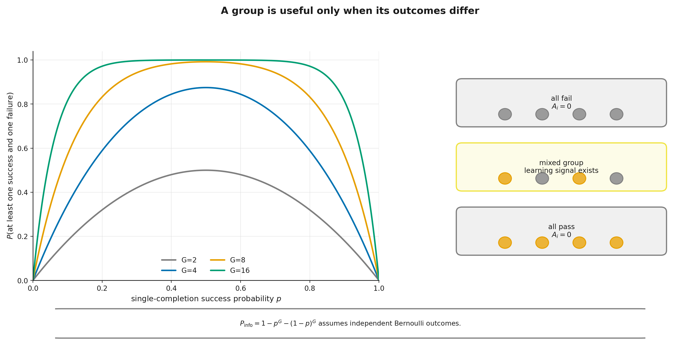
When , almost every group is all wrong; when , almost every group is all correct. The signal is strongest near .
For :
| 0.01 | 0.0773 |
| 0.10 | 0.5695 |
| 0.50 | 0.9922 |
| 0.90 | 0.5695 |
| 0.99 | 0.0773 |
To obtain informative prompts at an approximately stationary rate,
This motivates dynamic resampling and a moving difficulty curriculum. It also changes the training distribution: easy and nearly impossible prompts stop contributing gradients. Keep the original stream, rejection reason, and evaluation on the complete held-out distribution.
The formula assumes independent draws conditional on one fixed prompt and generation protocol. Low temperature, a fixed template, and independently repeated prefixes can reduce entropy while preserving independence. Reusing a sampled prefix or a search branch across candidates can couple draws. Across prompts, different success probabilities also matter: average the per-prompt formula rather than substituting a pooled success rate. Duplicate answers alone do not identify dependence.
Lesson 9.2. Canonical GRPO
Lesson 9.2. Canonical GRPO
- Three policies and one data source
- Group baseline and advantage estimate
- The clipped objective
- Why the first update may not need a nontrivial ratio
- Relationship to REINFORCE, RLOO, and PPO
then 3 assessment steps
Step 9.2.1 — Three policies and one data source
For prompt , the old policy samples a group
Three roles must then remain distinct:
- old policy — the actual source of stored actions and the denominator of importance ratios;
- current policy — the model whose gradient is being computed;
- reference policy — an optional KL anchor.
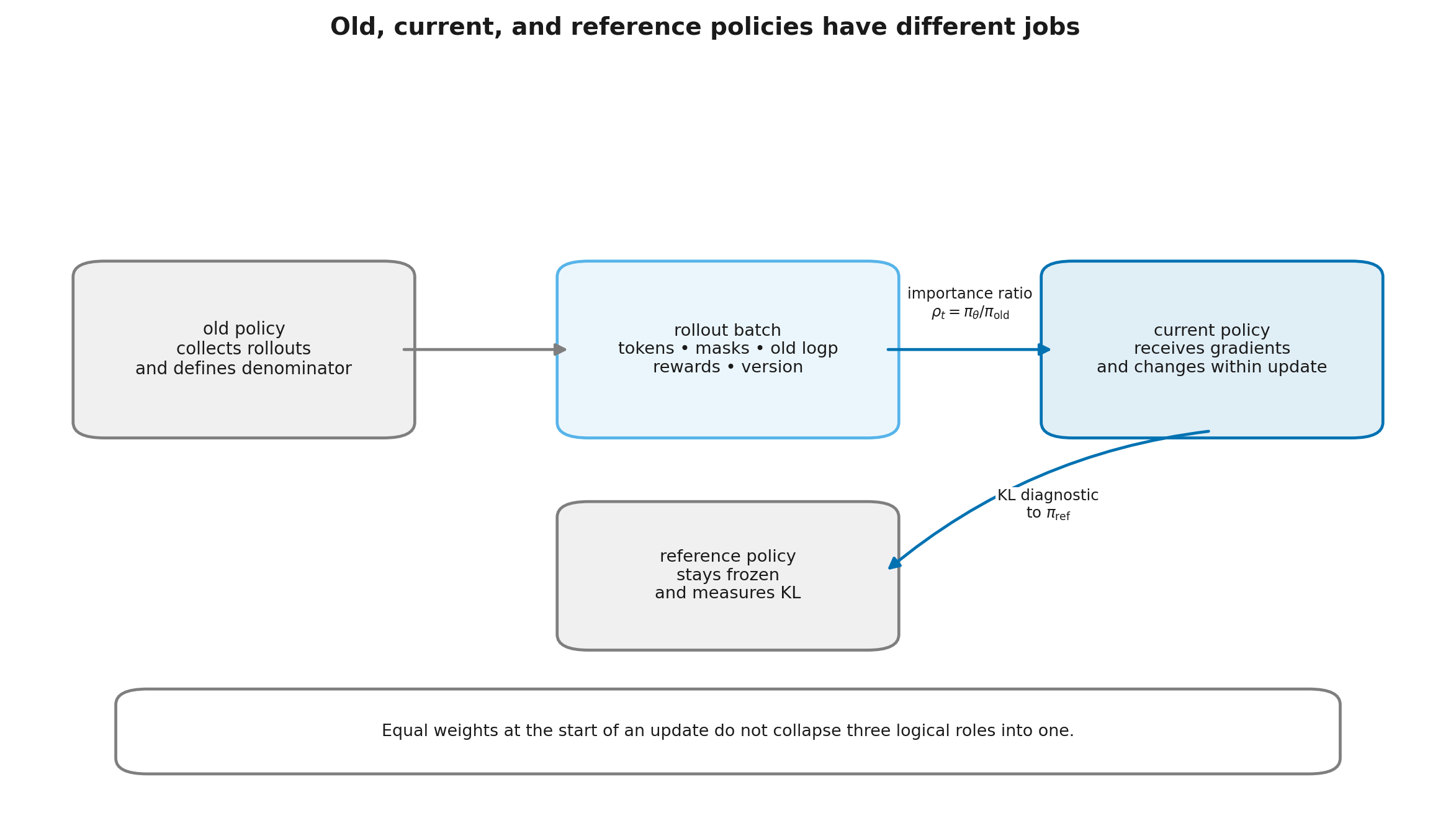
Old and reference policies may start from identical weights, but they are different mathematical objects. The old policy is frozen for a rollout batch and replaced when a new batch is collected. The reference may remain frozen, be replaced under an explicit schedule, or be omitted. The current policy changes while the batch is optimized.
For token , define
The denominator must describe the actual behavior policy after temperature, masks, top-k/top-p, and any other logit processing. If generation used a transformed distribution, raw-softmax log-probabilities cannot be substituted merely because they are easier to obtain. Stored old log-probabilities, decoding parameters, and the generator version belong in the rollout record.
Step 9.2.2 — Group baseline and advantage estimate
For rewards , canonical GRPO uses
where is the within-group standard deviation.
The same is usually applied to every token in response . This removes the learned value model, but it does not solve token-level credit assignment: every token in a successful response receives the same sign.
“GRPO has no baseline” is false. The group mean is a baseline. What GRPO removes is a learned critic that predicts state values.
For a binary group with one success and population standard deviation,
and every failure has
ignoring the numerical . The group estimates sum to zero, but their scale depends on group composition.
Step 9.2.3 — The clipped objective
The original DeepSeekMath presentation uses token-level ratios and averages token terms within each response before averaging responses:
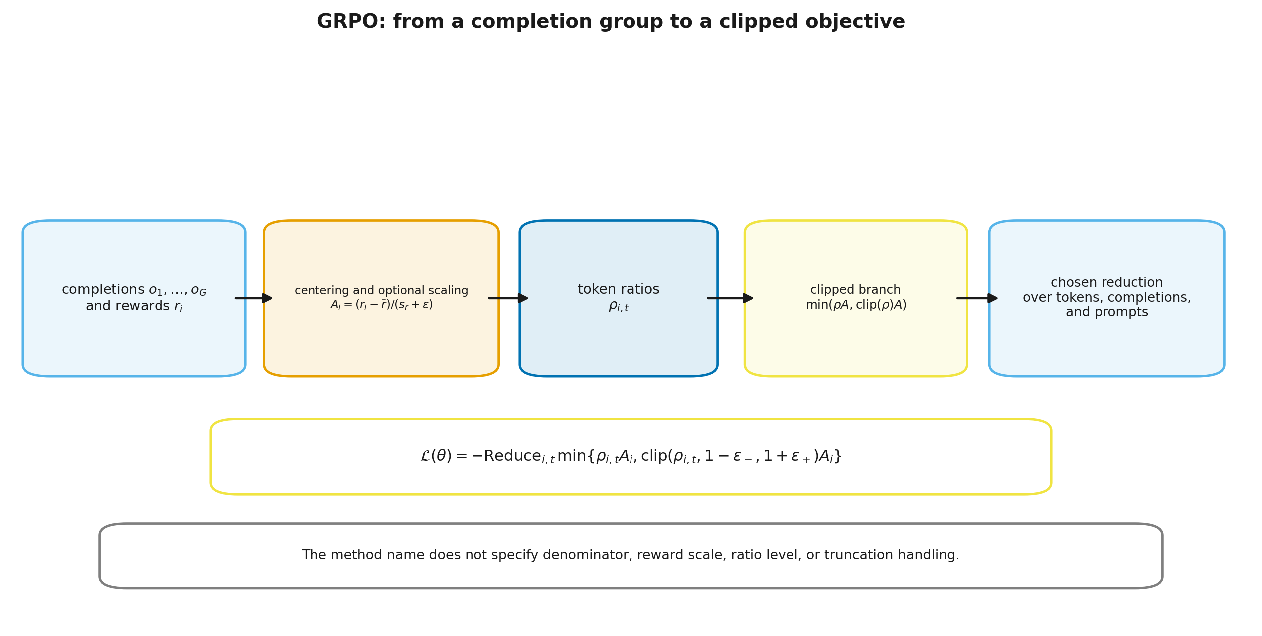
is the chosen estimator of deviation from the reference. Its exact form matters: a sampled log-ratio, a non-negative sample form such as , and the exact categorical KL have different variance, bias, and gradient contracts.
Clipping behaves differently for the two advantage signs:
- when , the upper branch stops further growth of the surrogate contribution after the ratio has increased too far;
- when , the lower branch limits the apparent gain from decreasing probability too aggressively;
- clipping does not project the policy into a trust region, force every into the interval, or impose a strict KL bound.
Notation differs across papers and libraries. DeepSeekMath uses token ratios; the DeepSeek-R1 report displays a compact sequence-level expression; current libraries expose several ratio levels and reduction schemes. The word GRPO therefore does not reconstruct an implementation. At minimum, specify the ratio unit, reduction denominator, epochs per rollout batch, truncation handling, and KL contract.
Step 9.2.4 — Why the first update may not need a nontrivial ratio
When rollouts were generated by the current weights and exactly one forward/backward pass occurs before any policy change,
at the evaluation point, so . The objective still has a policy-gradient derivative through current log-probabilities, but clipping is inactive.
Ratios matter after repeated mini-batches, several optimization iterations on the same completions, or asynchronous generator lag. The data then becomes progressively less on-policy.
A precise classification is:
- fresh responses and one update: effectively on-policy;
- several iterations over one rollout batch: near/on-policy with bounded reuse;
- large asynchronous lag or a long-lived buffer: off-policy, requiring separate analysis.
Log num_iterations, rollout age, generator checkpoint, and the ratio distribution. “We used GRPO” conveys none of these details.
Step 9.2.5 — Relationship to REINFORCE, RLOO, and PPO
Without clipping, KL, or rollout reuse, a group-mean baseline yields a REINFORCE-like estimator:
REINFORCE Leave-One-Out (RLOO) instead uses the mean of the other rewards for response :
Under conditionally independent sampling, this baseline is independent of the current action and avoids the finite-sample scaling induced by the common sample mean. GRPO generally retains the common group mean and adds normalization, clipping, and sometimes KL.
PPO uses a learned critic and stepwise advantage estimates. GRPO replaces the critic with comparisons among responses to the same prompt. That saves model memory while increasing dependence on rollout count, verifier quality, and within-group diversity.
Compact map: RLVR specifies where reward comes from; REINFORCE, RLOO, GRPO, and PPO specify how the gradient is estimated and applied.
Lesson 9.3. Normalization and algorithm variants
Lesson 9.3. Normalization and algorithm variants
- Dividing by group standard deviation reweights prompts
- Length normalization decides who receives gradient
- DAPO: four related but independent changes
- GSPO: an importance ratio for the whole response
- A method name is not a full specification
then 6 assessment steps
Step 9.3.1 — Dividing by group standard deviation reweights prompts
The normalization
makes the spread of each nondegenerate group approximately unit scale. That is convenient numerically, but it also changes the relative weight of prompts.
Consider centered rewards
and
The second group has ten times smaller differences. Dividing each by its own standard deviation makes the normalized advantages identical. A barely differentiated partial signal receives the same scale as a large reward gap.
Understanding R1-Zero-Like Training: A Critical Perspective calls this question-level difficulty bias and proposes Dr. GRPO with
and no within-group standard-deviation scaling.
This is not free. Without normalization, update scale depends directly on reward units and batch composition. Components in and cannot be combined without explicit calibration.
Step 9.3.2 — Length normalization decides who receives gradient
Original GRPO averages each response over its own tokens:
Each response therefore has length-independent total weight, while each token receives weight proportional to . A long failed response gets weaker negative pressure per token than a short failed response.
Dr. GRPO replaces the response-specific denominator with a fixed constant , such as the maximum completion length:
DAPO normalizes by the total number of active tokens:
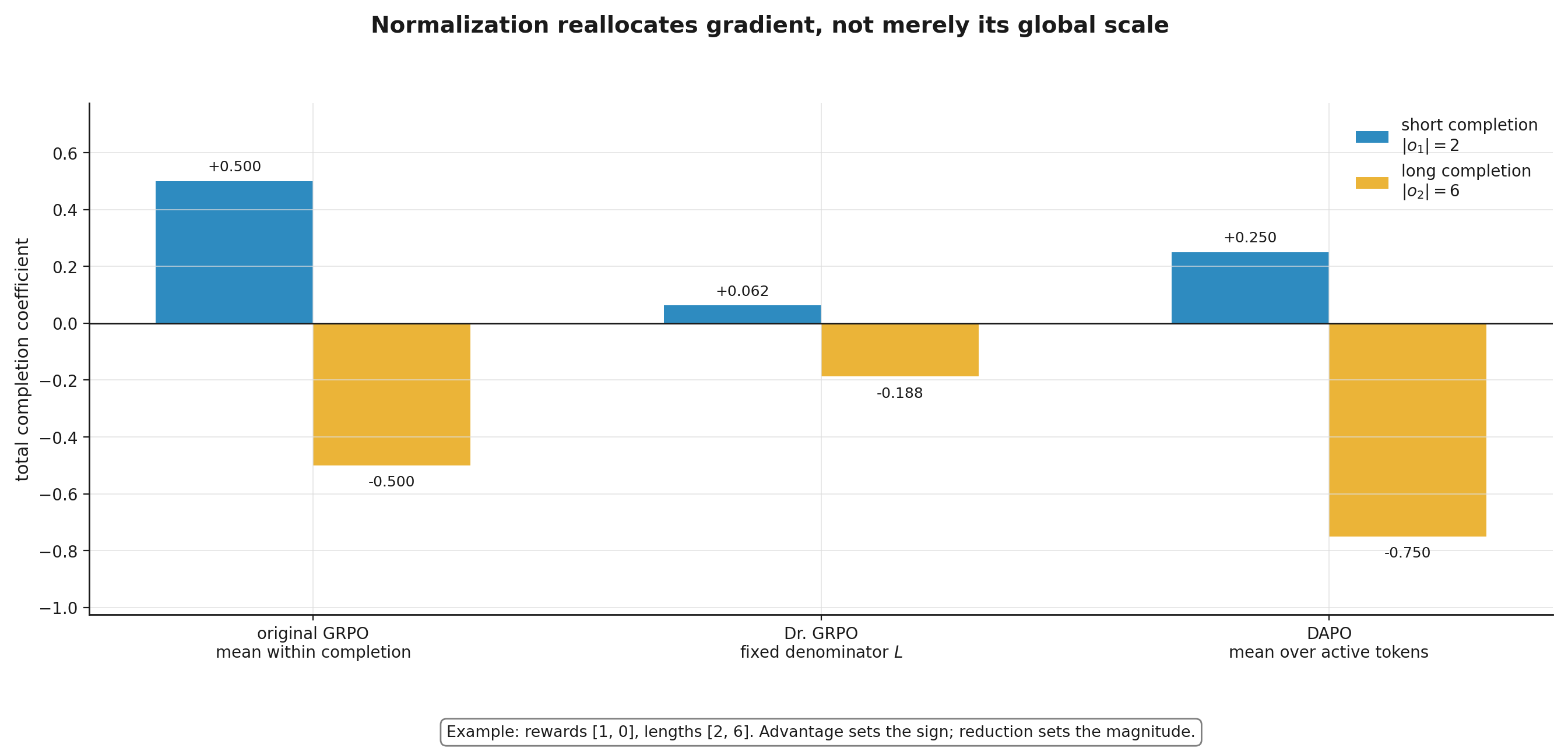
Both remove the per-response length denominator, but they are not identical. Dr. GRPO uses a denominator independent of random batch lengths; DAPO’s denominator changes with the active-token count. This can matter across distributed layouts and gradient accumulation schemes.
Neither objective proves that longer responses are useful. It only allocates gradient budget among tokens.
Step 9.3.3 — DAPO: four related but independent changes
Decoupled Clip and Dynamic sAmpling Policy Optimization (DAPO) combines four techniques.
- Clip-Higher. It separates the lower and upper ranges:
The authors argue that an early upper clip can suppress growth of rare but useful tokens. This is an empirical mechanism and stabilization choice, not a guarantee of diversity.
-
Dynamic sampling. All-equal reward groups are rejected and generation continues until enough informative prompts have been collected. The costs are additional tokens and a changed prompt distribution.
-
Token-level policy-gradient loss. All active tokens in the batch share one normalizer instead of averaging each response first.
-
Overlong reward shaping. The paper first evaluates masking truncated responses, then introduces the soft penalty
DAPO therefore cannot be summarized as “always drop truncated responses.” Masking was one investigated variant; the named package includes a gradual length reward near the boundary.
Step 9.3.4 — GSPO: a normalized response-level ratio
Group Sequence Policy Optimization (GSPO) changes the unit of correction. It uses one length-normalized response-level ratio:
The sequence-level term is clipped:
This is the geometric mean of token ratios, not the unnormalized product of full-sequence probabilities. The GSPO authors argue that the unit of correction and clipping should match the sequence-level reward. They report improved stability in the long-response and mixture-of-experts settings they studied. These are reported experiments, not a theorem of universal superiority.
Length normalization keeps the sequence ratio numerically manageable, but the gradient still flows through all token log-probabilities. GSPO clip ranges are not numerically interchangeable with token-level GRPO ranges because the ratios live on different scales.
Step 9.3.5 — A method name is not a full specification
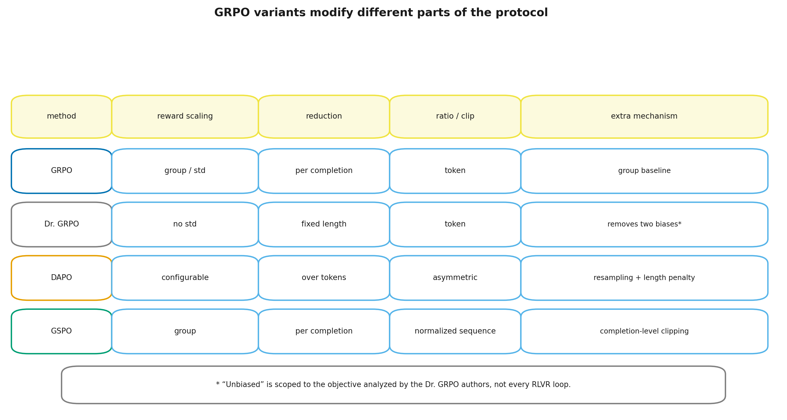
| Variant | Reward scaling | Token-term normalization | Ratio level | Additional choices |
|---|---|---|---|---|
| Original GRPO | group centering and standard deviation | per response length | token | symmetric clip, optional KL |
| Dr. GRPO | centering only | fixed constant | token | removes the two mechanisms identified by its authors |
| DAPO | usually group scaling | active tokens in batch | token | Clip-Higher, dynamic sampling, length shaping |
| GSPO | group-relative estimate | sequence objective | normalized response ratio | geometric-mean ratio and sequence clip |
Production code often creates hybrids: DAPO token normalization without standard-deviation scaling, asymmetric clipping with Dr. GRPO, or a sequence-level ratio with another reduction. Such a run cannot be described honestly by one acronym.
A minimum algorithm record includes:
- behavior-policy source and version;
- completions per prompt;
- reward-component aggregation;
- reward centering and scaling;
- probability-ratio level;
- clipping function;
- token, response, and device normalization;
- rollout-reuse iterations;
- KL estimator and coefficient;
- truncation masks and stop reasons.
Software snapshot on 2026-08-05. TRL 1.9.2 exposes these axes independently. Its GRPOConfig documentation lists, among other defaults:
loss_type="dapo"
scale_rewards="group"
importance_sampling_level="token"
beta=0.0
mask_truncated_completions=False
Other modes include loss_type="dr_grpo", batch-level reward scaling, sequence-level ratios, and explicit masking of truncated completions. These defaults describe one library release, not the mathematical definition of GRPO. A reproducible run stores the actual arguments instead of relying on remembered defaults from another version.
Lesson 9.4. Training dynamics and diagnosis
Lesson 9.4. Training dynamics and diagnosis
- Entropy: specify what is measured
- Loss of diversity and interventions
- Length, EOS, and technical truncation
- Elicitation of reachable behavior versus new effective strategies
- A minimum dashboard
then 5 assessment steps
Step 9.4.1 — Entropy: specify what is measured
For prefix , token entropy is
Logs typically average over active tokens and completions. A single mean hides structure: opening moves, operation choices, formatting tokens, and final-answer tokens may behave differently.
Distinguish:
- entropy of the base softmax;
- entropy of the actual behavior policy after sampling transforms;
- full-response diversity;
- semantic strategy diversity;
- held-out pass@k.
These quantities are related but not identical. High token entropy can be spent on punctuation; low entropy can encode a stable correct algorithm.
The 2025 paper The Entropy Mechanism of Reinforcement Learning for Reasoning Language Models reports, in its studied runs, rapid entropy reduction and a disproportionate update contribution from a minority of high-entropy tokens. A later 2026 preprint proposes an explicit on-policy entropy-flow mechanism to resist collapse. Both are useful sources of diagnostic hypotheses, but neither defines a universal “healthy entropy” threshold across models, rewards, and response lengths; the 2026 result should additionally be treated as recent frontier evidence rather than settled theory.
Step 9.4.2 — Loss of diversity and interventions
Warning signs include:
- entropy falls without stabilizing;
- responses within a group become near duplicates;
- informative-group rate falls faster than accuracy alone explains;
- pass@1 rises while the pass@k curve stops improving;
- upper clip fraction and heavy-tailed ratios grow;
- different random seeds converge to the same response template.
Possible interventions are:
- increase diversity of the actual behavior policy;
- widen the positive upper clip;
- add cautious entropy regularization;
- increase or prompt diversity;
- move the difficulty band;
- reduce rollout-reuse iterations;
- stop before severe collapse;
- separate reward components when one dominates.
Every intervention has a cost. More sampling temperature can lower correctness and raise generation expense. An entropy bonus rewards useful and useless uncertainty. Larger costs more generation. Clip-Higher relaxes one constraint but cannot repair a wrong reward.
Step 9.4.3 — Length, EOS, and technical truncation
A growing mean response length may indicate:
- useful additional reasoning steps;
- weak per-token penalties for long failures;
- repetition encouraged by format or reward;
- decreasing probability of the end-of-sequence (EOS) token;
- a rising fraction of responses cut by the length limit.
Log length together with:
- reward or correctness by length bucket;
- natural termination and truncation rates;
- EOS position;
- length after removing control tags;
- repetition and parse-failure rates;
- generation cost.
A truncated response is not necessarily wrong: the checker did not observe its ending. Unconditionally ignoring every truncated response is also unsafe because the policy may learn to avoid negative feedback by never stopping. Choose and record a contract: masking, a soft penalty, a separate label, or a larger budget.
The target is not “longer” or “shorter” responses. It is better quality under a declared budget and an interpretable stopping process.
Step 9.4.4 — Elicitation of reachable behavior versus new effective strategies
A large pass@1 increase after RL does not by itself explain the source of improvement.
One hypothesis is that the policy reweighted successful trajectories that the base model could already produce under a sufficiently large sampling budget. This is elicitation of practically reachable behavior. Another is that training made strategies practically reachable that were essentially absent under the original budget. This is new effective strategy discovery.
Use “support” carefully. A standard softmax gives most tokens nonzero probability. The operational object is effective support under fixed temperature, maximum length, and sampling budget.
A minimum comparison protocol is:
- plot base and RL pass@k curves under identical decoding;
- compare strategy clusters, not only final answers;
- use fresh tasks and contamination controls;
- repeat across random seeds;
- separate RL effects from later SFT or distillation.
A 2025 study concludes that, for the models and tasks it examined, much of the gain could be explained by reweighting trajectories already reachable from the base model. This is an important counterweight to strong “reasoning creation” claims, not a final answer for all scales and domains.
The full treatment of Best-of-N, self-consistency, and search is in Module 10 “Search, verification, and test-time compute” (rl_llm.module_10_test_time_search).
Step 9.4.5 — A minimum dashboard
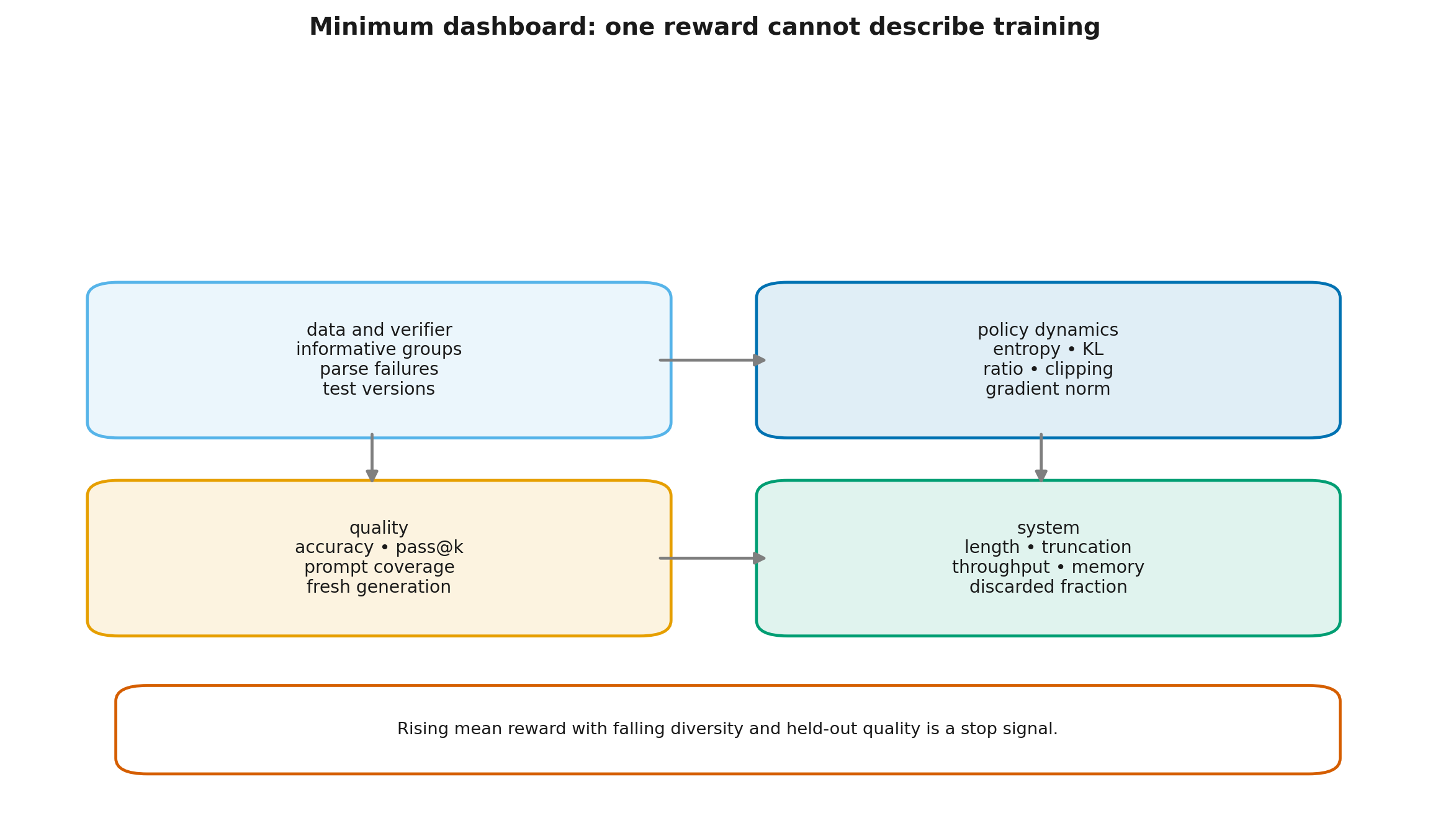
A group-based RLVR dashboard needs several independent axes.
Data and verification
- every reward component separately;
- parse errors, timeouts, and exceptions;
- informative-group fraction;
- reward distributions by source and difficulty.
Policy and optimization
- average and position-wise entropy;
- KL to the declared reference, when computed;
- token- or sequence-ratio distribution;
- positive and negative clip fractions separately;
- rollout age and reuse count.
Responses and quality
- pass@1 and several pass@k points on held-out data;
- mean, median, and tail length;
- EOS, truncation, and parse-failure rates;
- string and semantic-strategy diversity;
- performance on control tasks outside the training domain.
System
- generated tokens per informative prompt;
- generation and optimization time;
- peak memory;
- stale or reused rollout fraction.
Define stopping criteria before training, such as no independent-quality improvement while proxy reward keeps rising, a sharp pass@k decline, or a growing checker-error rate.
Lesson 9.5. From formulas to a reproducible run
Lesson 9.5. From formulas to a reproducible run
- Data and verifier passport
- Rollout and update passport
- Resource profiles and the absence of a universal recipe
- Lab: synthetic loop and optional real-model GRPO
- Summary and module boundary
then 8 assessment steps
Step 9.5.1 — Data and verifier passport
Before the first update, record:
- prompt provenance and train/evaluation split rules;
- reference-answer provenance and license;
- verifier version;
- false-positive and false-negative rates on a manually reviewed sample;
- initial pass-rate distribution;
- answer format and chat template;
- stopping rules;
- length and execution limits;
- handling of ambiguous or damaged examples.
Code tasks additionally require container image, compiler, dependencies, network policy, time, memory, and test determinism. Formal mathematics needs kernel version and allowed axioms. Numerical tasks need canonicalization and tolerances.
Dynamic sampling must not erase the original distribution. Keep accepted and rejected prompts with rejection reasons.
Step 9.5.2 — Rollout and update passport
A rollout batch should reproduce the loss without regenerating outputs. Minimum fields are:
- prompt identifier and tokens;
- completion tokens and action mask;
- log-probabilities under the actual old policy;
- generator checkpoint/version;
- decoding parameters and random seed;
- reward components;
- parse result and stop reason;
- length before and after truncation;
- reference log-probabilities when needed;
- group identifier and completions per prompt.
The update passport adds:
- reward centering and scaling;
loss_typeand exact denominator;- importance-ratio level;
- clip ranges;
- iterations per batch;
- KL and entropy coefficients;
- global batch size and gradient accumulation.
Generator and trainer distributions may differ even with the same checkpoint identifier because of library versions, precision, logit processors, and templates. Measure this mismatch rather than assuming it is zero.
Step 9.5.3 — Resource profiles and the absence of a universal recipe
Level A: CPU. NumPy reference functions, verifier tests, synthetic groups, comparison of normalization, clipping, and sequence ratios. This path is required for understanding and uses no language model.
Level B: free Colab T4. A roughly 0.6B model, LoRA, short completions, few generations, and an explicit smoke configuration. The goal is to observe the data path, not reproduce a large technical report.
Level C: optional full run. A larger model, long completions, a separate rollout engine, multiple GPUs, and reproducible infrastructure. Cost depends on completion length, group size, reuse, and verification expense.
Do not copy , , , temperature, or learning rate as an “R1 recipe.” They interact with model size, reward scale, sequence length, batch size, optimizer, and loss normalization. Changing the denominator changes effective gradient scale.
Step 9.5.4 — Practice: an autoregressive CPU loop and an optional real model
Practice is split by language:
The core route runs on CPU and uses a small but genuine autoregressive model: an embedding layer, a GRU, and a language-model head. Responses are generated token by token under a constrained grammar. The versioned verifier returns correctness, intermediate consistency, format status, and total reward separately. Each prompt receives a group sampled by the frozen old policy; the current policy is then optimized with a clipped group-relative objective. A separate reference policy is retained for teacher-forced KL diagnostics.
The loop is small in scale but realistic in contract. It exposes:
- the actual behavior distribution after the allowed-token mask;
- reproduction of stored old log-probabilities under the frozen old policy;
- group advantages and the zero signal of an all-equal group;
- multiple update epochs over one rollout batch;
- entropy, clipping, length, KL, and informative-group rate;
- fresh-generation evaluation rather than training loss alone;
- held-out arithmetic prompts and prompt-level coverage.
The course’s fixed smoke profile produced:
| Metric | Before RL, train | After RL, train | Before RL, held-out | After RL, held-out |
|---|---|---|---|---|
| accuracy | 0.313 | 0.408 | 0.033 | 0.000 |
| mean reward | 0.341 | 0.448 | 0.037 | 0.000 |
| mean length | 7.03 | 8.38 | 6.92 | 9.24 |
| token entropy | 0.292 | 0.148 | 0.382 | 0.285 |
| teacher-forced KL to reference | 0.000 | 0.219 | 0.000 | 0.195 |
| pass@4 | 0.583 | 0.450 | 0.111 | 0.000 |
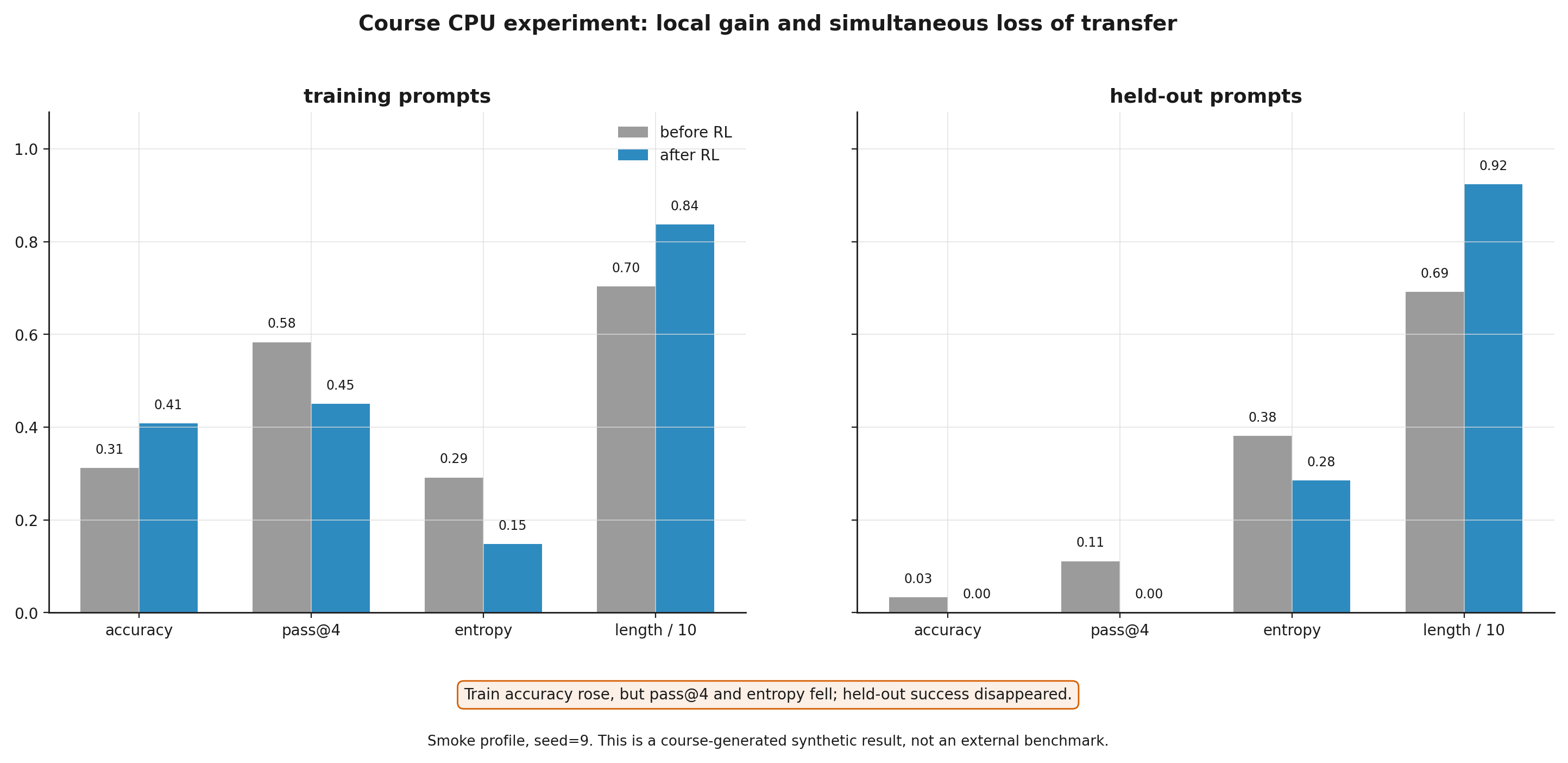
This is a course-generated synthetic result, not an external benchmark. Mean training accuracy rose, yet entropy and pass@4 fell, successes concentrated on fewer training prompts, and transfer to held-out combinations vanished. One mean reward is therefore not sufficient evidence of a good update. The small experiment does not claim that GRPO must collapse; it reproducibly demonstrates a failure pattern that a serious evaluation stack must be able to detect.
The optional real-model branch is disabled by default:
RUN_REAL_MODEL = False
SMOKE_MODE = True
Its configuration skeleton targets Qwen/Qwen3-0.6B, LoRA, and GRPOTrainer. The snapshot pins TRL 1.9.2, Transformers 5.14.1, Datasets 5.0.1, PEFT 0.20.0, Accelerate 1.14.0, and bitsandbytes 0.50.0. This branch was not executed in the release gate: no runtime, memory use, or quality result is claimed for it. Before a Colab run, re-check the current CUDA image, model, package compatibility, and every GRPOConfig argument.
Step 9.5.5 — Conclusions and boundaries
The main conclusions are:
- RLVR is a feedback regime; GRPO is a family of policy updates. Neither defines the other.
- A verifiable reward remains a proxy. Parsing, canonicalization, tests, and execution environment belong to the training contract.
- Canonical GRPO replaces a learned critic with a group baseline but does not solve within-response credit assignment.
- Old, current, and reference policies have different roles. The ratio denominator must match the actual behavior policy.
- Group-standard-deviation and per-response-length normalization are not neutral: they allocate weight across prompts and tokens.
- Dr. GRPO, DAPO, and GSPO modify different parts of the protocol; comparison requires the complete objective and reduction.
- Entropy, response diversity, pass@k, and informative-group rate are distinct diagnostics.
- Longer output does not prove better reasoning, and truncation is not identical to an incorrect answer.
- Elicitation-versus-discovery claims require matched sampling budgets and analysis of the trajectories themselves.
- A smoke run proves that the loop executes; it does not reproduce a large-scale paper result.
Continuation within this course:
- Module 10 “Search, verification, and test-time compute” (
rl_llm.module_10_test_time_search) develops Best-of-N, self-consistency, and search; - Module 12 “RL infrastructure for LLMs: memory, rollouts, and asynchrony” (
rl_llm.module_12_infrastructure) covers distributed generation, policy versions, and rollout economics; - Module 13 “Evaluating RL systems for LLMs: statistics, reward hacking, and safety” (
rl_llm.module_13_evaluation) builds the statistical and safety evaluation stack.
Extensions in the companion courses:
- Modern LLMs, Module 14 “Learning from Feedback: RLHF, DPO, RLOO, and GRPO” (
modern_llms.module_12_preference_optimization) provides the broader post-training context; - Modern LLMs, Module 15 “Reasoning Models and Test-Time Compute” (
modern_llms.module_13_reasoning) connects RLVR to reasoning-model architectures and inference budgets; - Information Theory for ML, Module 2 “Entropy” (
it_ml.module_02_entropy) develops entropy formally; - Information Theory for ML, Module 3 “Cross-Entropy and KL Divergence” (
it_ml.module_03_cross_entropy_kl) treats KL as a divergence between distributions; - Information Theory for ML, Module 8 “Maximum entropy, exponential models, and KL regularization” (
it_ml.module_08_maxent_kl_policy) gives the variational view of KL-regularized policy updates.
These references deepen selected topics, but Module 9 remains self-contained: every definition and equation required by its exercises and practice is introduced here.
Sources and reading route
- DeepSeekMath: Pushing the Limits of Mathematical Reasoning in Open Language Models — the original GRPO presentation and token-level clipped objective.
- DeepSeek-R1: Incentivizing Reasoning Capability in LLMs via Reinforcement Learning — R1-Zero, rule-based rewards, and the final multi-stage pipeline.
- Understanding R1-Zero-Like Training: A Critical Perspective — the normalization, response-length, and question-difficulty analysis behind Dr. GRPO.
- DAPO: An Open-Source LLM Reinforcement Learning System at Scale — Clip-Higher, dynamic sampling, token-level reduction, and overlong reward shaping.
- Group Sequence Policy Optimization — a response-level unit for the ratio and clipping decision.
- The Entropy Mechanism of Reinforcement Learning for Reasoning Language Models — empirical and mechanistic entropy analysis in the authors’ studied runs.
- Does Reinforcement Learning Really Incentivize Reasoning Capacity in LLMs Beyond the Base Model? — evidence on eliciting practically reachable trajectories; its conclusions are not universal across models and regimes.
- TRL GRPOTrainer documentation — the current engineering interface, not a primary source of mathematical guarantees.
The complete claim registry, including the precise status of course-generated experiments, is in Module_9_Sources.md.