Module 5. Learning from fixed data: imitation, deep Q-methods, and offline RL
Material version: 2026.10
Factual snapshot: 2026-08-05
Language: EN
Core practice: NumPy for local calculations plus a separate English PyTorch notebook with a self-contained KeyDoorGrid environment, BC, DAgger, DQN, Double DQN, a BCQ-like constraint, CQL, IQL, FQE, Decision Transformer, and a token-level ILQL-like pipeline
Structure: 5 lessons, 25 steps
Estimated time: 9–13 hours including the main notebook; the full experiment profile is optional
In Module 4, the policy improved from trajectories that it collected itself. We now forbid new interaction during optimization. All that remains is a fixed collection of demonstrations, logged transitions, rewards, or preference pairs, and we must determine what can actually be learned from it.
This is a fundamental change rather than a minor engineering choice. Fixed data can make learning cheaper and safer, but the algorithm can no longer test its own guesses. If an action never appears in the log, its consequences may be unknown not because the neural network is insufficiently capable, but because the data do not identify the answer.
No prior course in classical RL is required. We begin with imitation learning and the exact relation between behavioral cloning (BC) and supervised fine-tuning (SFT), then study the deep Q-network, formulate the central difficulty of offline RL, compare several method families, and finish with Decision Transformer and a data-centric map of LLM post-training methods.
Learning objectives. By the end of the module, you will be able to:
- write behavioral cloning as maximum likelihood and state when token-level SFT is a special case;
- distinguish the expert state distribution from the distribution induced by the learned policy;
- derive the exact loss in a simple tightrope problem and explain the worst-case quadratic dependence on horizon;
- describe Dataset Aggregation (DAgger) without confusing expert action labels with preferences or scalar rewards;
- construct the Deep Q-Network (DQN) target and explain the distinct roles of replay memory and the target network;
- compute a Double DQN target and identify the source of maximization bias;
- distinguish offline RL from ordinary off-policy learning and from behavioral cloning;
- formulate the data-coverage problem and prove a simple impossibility result for an unobserved action;
- explain Batch-Constrained Q-learning (BCQ), Twin Delayed Deep Deterministic Policy Gradient plus behavioral cloning (TD3+BC), Conservative Q-Learning (CQL), and Implicit Q-Learning (IQL) without claiming universal superiority;
- describe Decision Transformer as a conditional sequence model and correctly update a desired return-to-go;
- separate SFT, classical offline RL, Direct Preference Optimization (DPO), Implicit Language Q-Learning (ILQL), and online policy optimization for LLMs.
The graded practice places every task next to a worked solution inside a `` block. The English and Russian executable routes share a computational core and use independently written explanations. Verified claims and primary sources are registered in Module_5_Sources.md.
The practical thread uses a single compact environment, KeyDoorGrid. The agent starts from several cells, must collect a key, pass a locked door, and reach the goal while avoiding traps. A trap is a true terminal; an external step limit merely truncates data collection. Reusing one environment connects demonstrations, DAgger, DQN, a fixed offline log, policy evaluation, and conditional trajectory modeling without pretending that their objectives are identical.
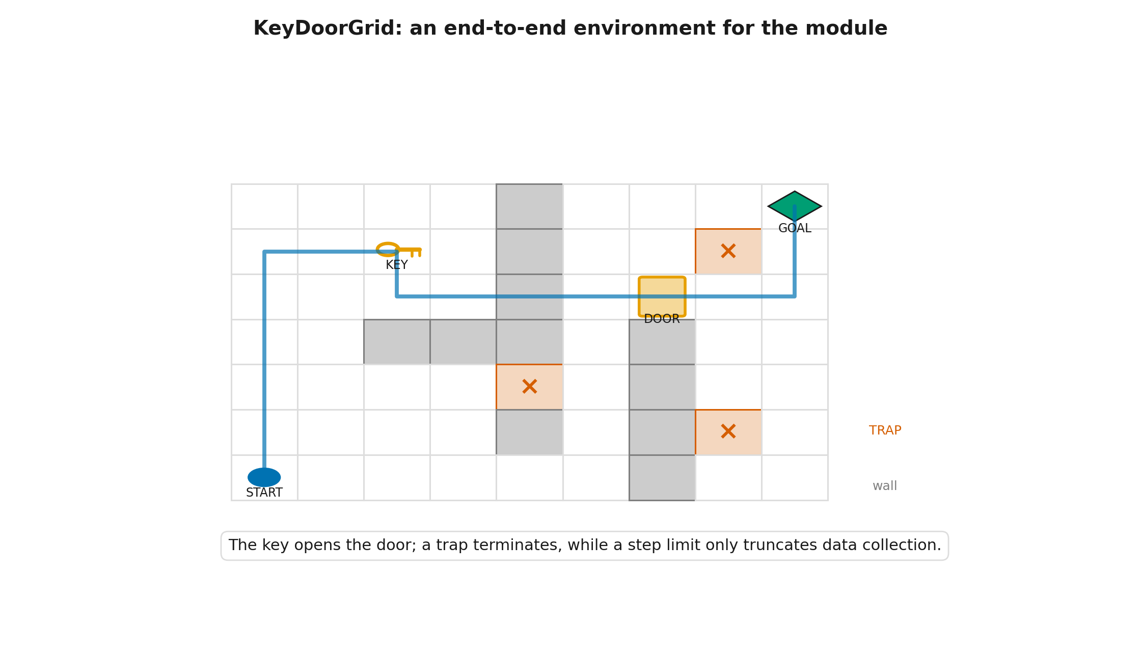
Practice route. Graded tasks, worked solutions revealed after an attempt, and executable practice follow the lecture. The explanation remains self-contained.
Lesson 5.1. Imitation learning and SFT
Lesson 5.1. Imitation learning and SFT
- Demonstrations instead of reward
- Dataset prefixes during training, model prefixes during generation
- Tightrope: an exact compounding-error calculation
- DAgger: label the states visited by the learner
- What BC explains in LLM post-training, and what it does not
then 6 assessment steps
Step 5.1.1 — Demonstrations instead of reward
Begin with the simplest fixed data: an expert showed what to do but did not provide a reward function. A demonstration set contains pairs
where is a state visited by the expert and is the action selected there.
BC trains a parameterized policy to predict the expert action:
This is ordinary maximum likelihood. With discrete actions it is equivalent to minimizing cross-entropy. Reward, value functions, and Bellman equations do not appear in the objective.
Now translate the notation to an LLM. Let a demonstration contain a prompt , a response , and a mask that is one only for tokens included in the loss. Then
Under the token-level abstraction and , this is BC on expert prefixes. The qualification matters: the equality depends on the unit of action, the construction of the prefix, and the mask. If system tokens, user messages, or tool outputs are also trained on, the objective is still maximum likelihood, but it clones a broader sequence-generation process.
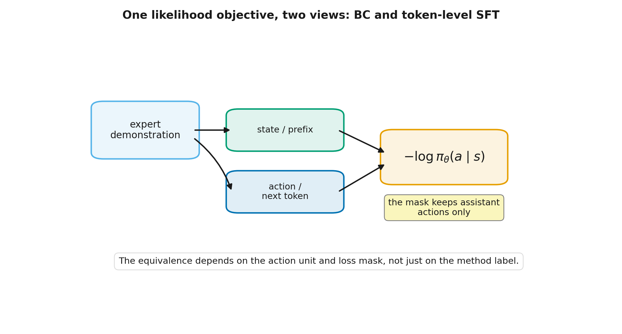
Demonstration preparation, sequence packing, masking, and the complete SFT pipeline are developed in Modern LLMs, Module 13 “Supervised Fine-Tuning and Data Work” (modern_llms.module_11_sft). Tokenization, special tokens, and message boundaries are covered in Modern LLMs, Module 2 “Tokenization and Embeddings” (modern_llms.module_02_tokenization). Both references are optional here: the algorithmic fact needed in this module is narrower—training observes demonstrator actions in states generated by the demonstrator.
For a deeper treatment of negative log-likelihood, cross-entropy, and KL divergence, see Information Theory for ML, Module 3 “Cross-Entropy and KL Divergence” (it_ml.module_03_cross_entropy_kl).
Step 5.1.2 — Dataset prefixes during training, model prefixes during generation
During training, a token model receives the correct preceding prefix from the dataset. This is teacher forcing. During generation, the next input contains the model's own tokens.
Let be the state distribution at time under the expert and the distribution under the learned policy. A standard BC error is measured on expert states:
Deployment quality, however, depends on states visited by the learned policy: .
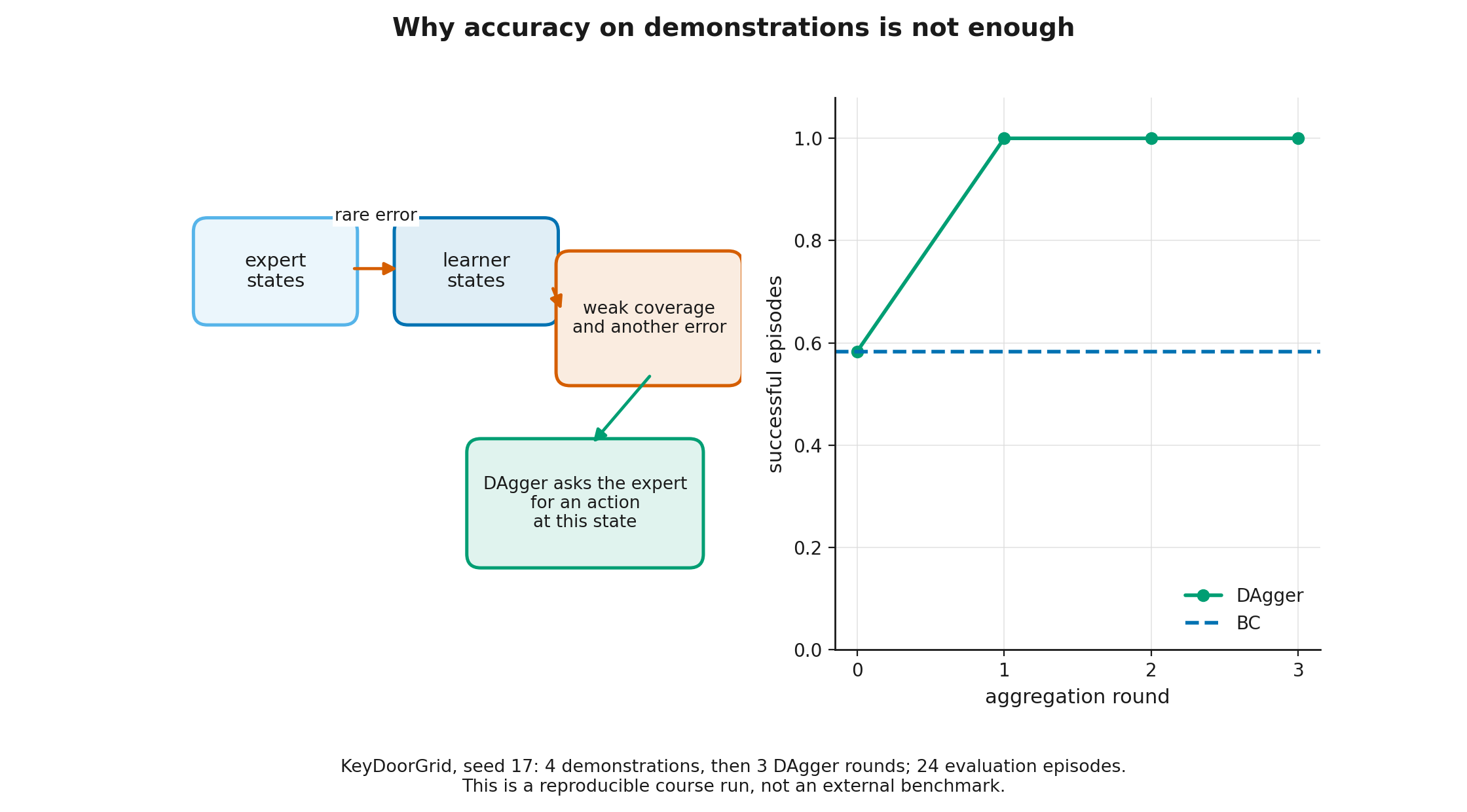
After the first mistake, the two distributions may diverge. The policy enters a state that rarely occurred in demonstrations, makes a larger error there, and moves farther away. In sequential prediction this is called compounding error; in autoregressive modeling the train–generation mismatch is often called exposure bias.
A careful boundary is important. Distribution shift does not prove that every long generation must fail. The model may generalize to novel prefixes, and an error may be recoverable. The precise statement is:
Small error on the expert-state distribution does not by itself guarantee small error on the state distribution induced by the learned policy.
This separates predictive accuracy from closed-loop policy quality.
Step 5.1.3 — Tightrope: an exact compounding-error calculation
Consider a deliberately simple task. The expert survives steps and earns at every successful step. On each step before failure, the imitator independently makes an error with probability . After the first error all subsequent rewards are zero.
The probability of receiving the reward at step is , so the expected return is
For ,
The expert earns , hence
When , the expansion gives
The leading dependence is . An early error can cost the entire remaining suffix, not just one reward.
This is not a universal law for every environment. It isolates a worst-case mechanism in an irreversible task. Recoverable errors can cost less; errors that lead into increasingly dangerous states can cost more. The practical question is therefore not only “How accurate is the policy on demonstrations?” but also “What does an error cost, and can the policy recover from states that it creates itself?”
Step 5.1.4 — DAgger: label the states visited by the learner
Dataset Aggregation (DAgger) changes the training-state distribution.
- Train an initial policy on expert demonstrations.
- Run the current policy, or a mixture of the current policy and the expert.
- Collect the states actually visited by the learner.
- Ask the expert for the correct action in each collected state.
- Add the new pairs to the aggregated dataset and retrain.
- Repeat.
Instead of one supervised problem under , DAgger creates a sequence of problems whose states are tied to learner behavior. The original paper reduces this process to no-regret online learning. With a bounded cost-to-go difference and small average regret of the underlying learner, the additional cost scales as rather than the standard worst-case bound for naive BC.
That sentence is meaningful only together with its assumptions. The cost-to-go bound, online-learning regret, number of iterations, expert–learner mixture, and rule for selecting the final policy all enter the theorem. One extra DAgger round does not automatically repair arbitrary representation error or every environment.
In the course run, an initial BC policy trained on only four KeyDoorGrid demonstrations solved 14 of 24 evaluation episodes. After one DAgger round labeled learner-visited states, it solved all 24 and retained that rate in later rounds. This single-seed synthetic run illustrates the mechanism; it is not an external performance claim. The exact protocol is stored in data/M5_experiment_protocol.json.
DAgger is also not the same as reinforcement learning from human feedback (RLHF). DAgger asks an expert for the action that should be taken in a particular state. RLHF more often obtains a comparison, rating, or preference over whole responses. Both collect feedback on behavior produced by the current policy, but the signal and objective differ.
Step 5.1.5 — What BC explains in LLM post-training, and what it does not
Token-level SFT inherits both strengths and limitations of BC.
What it does well:
- transfers the style and format of demonstrations;
- introduces useful behavior without defining a reward;
- uses a stable and scalable likelihood objective;
- can preserve the base model's knowledge when data and optimization are chosen carefully.
Where the limitation appears:
- training prefixes come from demonstrations, while generation prefixes come from the model;
- recovery behavior may be rare in the dataset;
- equally plausible actions are not ranked by external utility unless that ranking is represented in the demonstrations;
- BC fits the conditional action distribution in the data rather than maximizing a separately specified reward.
RL after SFT is therefore useful for more than distribution shift. It can exploit verifiable rewards, preferences, interaction, and exploration. Conversely, every post-training pipeline need not begin with a new SFT stage: a base model may already be sufficiently prepared for the target signal.
A useful boundary is:
BC asks, “What would the demonstrator do in this state?” RL asks, “Which action improves the expected outcome under the chosen reward?”
The answers may coincide, but they need not.
Lesson 5.2. DQN: Q-learning with a neural network
Lesson 5.2. DQN: Q-learning with a neural network
- From a Q-table to a deep Q-network
- Experience replay
- The target network: a slower right-hand side
- Maximization bias and Double DQN
- The deadly triad and the boundary of the LLM analogy
then 3 assessment steps
Step 5.2.1 — From a Q-table to a deep Q-network
Module 2 updated a tabular estimate through
A table is impossible for images, long observations, or enormous state spaces. A Deep Q-Network (DQN) replaces it with . For a discrete action space, the network commonly maps one state to a vector of values, one per action.
For a transition , construct
where only for a true terminal transition and denotes a separate target network. Then minimize, for example,
Data collection usually uses an -greedy policy:
This remains Q-learning because the target maximizes over the next action rather than using the action actually selected by the behavior policy.
Step 5.2.2 — Experience replay
Adjacent transitions are strongly correlated: nearby frames look alike and the policy may remain in one part of the environment for many steps. DQN stores transitions in an experience replay buffer and trains on randomly sampled mini-batches.
The buffer has three practical roles:
- a transition can be reused in multiple updates;
- shuffling reduces short-range correlation within a mini-batch;
- data from several recent policy versions are mixed, making the update off-policy.
Replay does not turn DQN into offline RL. Standard DQN continues interacting with the environment and adds new transitions, so it can eventually repair missing coverage. Offline RL receives a fixed dataset; an absent action cannot be tried later.
Nor does random sampling make transitions strictly independent and identically distributed. They still arise from one dynamical system and a changing collection process. Replay merely makes the optimization stream less locally correlated.
Step 5.2.3 — The target network: a slower right-hand side
If one network supplies both and the target , every update moves both sides of the equation. The learner aims at a target that moves immediately with the prediction.
DQN maintains a second network . Its parameters are either copied periodically,
or updated by a slow moving average. Over several optimization steps the target changes more slowly than .
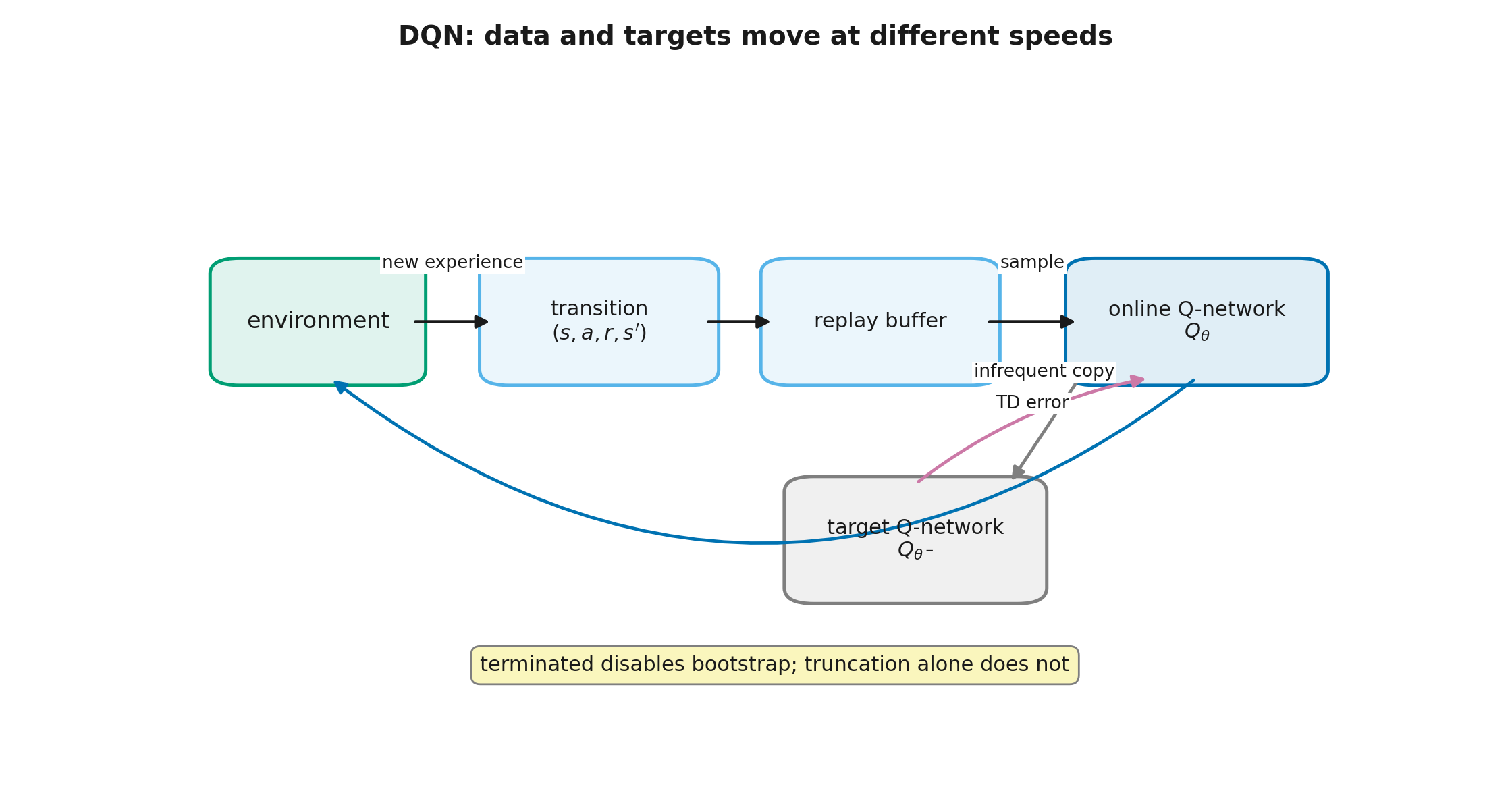
The DQN target network and an RLHF reference model may both be frozen copies, but their mathematical roles differ.
- The DQN target network supplies a bootstrapped value on the right-hand side of a Bellman target and is updated periodically.
- The RLHF reference policy defines a distance or regularization term, such as a Kullback–Leibler (KL) penalty, and is not a future-return estimate.
The same engineering pattern does not imply the same objective.
Step 5.2.4 — Maximization bias and Double DQN
Suppose two actions have equal true values but noisy estimates:
Even if each estimate is unbiased, their maximum is usually high:
The maximum tends to select whichever action received favorable positive noise. Bootstrapping can then propagate the overestimate backward.
Double DQN separates action selection from action evaluation:
The online network selects the action and the target network evaluates it. Their errors are not fully independent, but this separation reduces the systematic overestimation observed in DQN.
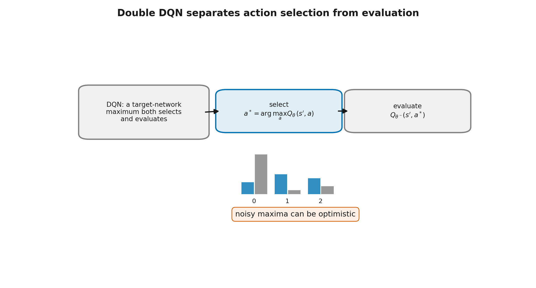
Double DQN does not eliminate every form of bias. Underestimation, correlated errors, and approximation error remain possible. It addresses one specific mechanism: using the same noisy estimator to choose a maximum and to evaluate that maximum.
Step 5.2.5 — The deadly triad and the boundary of the LLM analogy
Approximate Q-methods combine:
- neural function approximation;
- bootstrapping from their own estimates;
- off-policy data collected by another policy.
This combination is known as the deadly triad because it can produce divergence or severe instability. The slogan should not be inverted into “any two elements are always safe.” Convergence still depends on the algorithm, representation, data distribution, step sizes, and other assumptions.
A value-based approach to an LLM is mathematically possible: a token is a discrete action and a prefix is a state. Yet the action space is large, states almost never repeat exactly, rewards often arrive only after a whole response, and a strong pretrained policy already exists. Directly optimizing the autoregressive policy, or using it to constrain candidate actions, is therefore often more convenient.
This is an engineering preference, not a theorem of impossibility. Lesson 5.5 introduces ILQL, a value-based offline method for text generation.
The notebook implements DQN and Double DQN with replay, a target network, -greedy collection, separate termination and truncation flags, and a small replay warm-start from noisy expert-guided trajectories. In the pinned seed=5 run, after 130 episodes, DQN solved 20 of 24 evaluation episodes and Double DQN solved all 24. This verifies the end-to-end mechanics and exposes the target difference; it is not evidence of universal Double-DQN superiority. Another seed, replay composition, or exploration schedule can reverse the ranking.
Lesson 5.3. Offline RL: what can be learned from a fixed log
Lesson 5.3. Offline RL: what can be learned from a fixed log
- A fixed transition dataset
- Impossibility without coverage: two worlds, one dataset
- Extrapolation error and a self-reinforcing loop
- Four protection mechanisms for out-of-data actions
- Dataset quality, evaluation, and model selection
then 4 assessment steps
Step 5.3.1 — A fixed transition dataset
In offline reinforcement learning (offline RL), we receive
collected by one or more behavior policies . No new interaction with the environment is allowed during training. The goal is still to build a policy with high expected return.
| Setting | Data | Objective | New data during training? |
|---|---|---|---|
| BC | demonstrator states and actions | demonstrator action likelihood | not required |
| ordinary off-policy RL | transitions and rewards in a replay buffer | return | yes |
| offline RL | fixed transitions and rewards | return | no |
Offline RL tries to improve beyond average logged behavior by using action consequences and multi-step structure. Such improvement is possible only under sufficient coverage and appropriate assumptions about generalization. A reward label does not turn an absent transition into an observed one.
Step 5.3.2 — Impossibility without coverage: two worlds, one dataset
Consider one state and two actions, and . The log contains one thousand instances of with reward zero. Action never appears.
At least two environments are consistent with the data:
- world A: ;
- world B: .
The observed dataset is identical in both worlds. Any algorithm that sees only this dataset must return the same output for both, so it cannot both select the optimal action in A and avoid the harmful action in B with a universal guarantee.
This is not a failure of a particular neural network or of computation. It is non-identifiability: the answer is absent from the observations.
In a sequential task, an out-of-coverage action is evaluated through generalization. A maximum or actor may prefer an overestimate, and bootstrapping can propagate that error to earlier states.
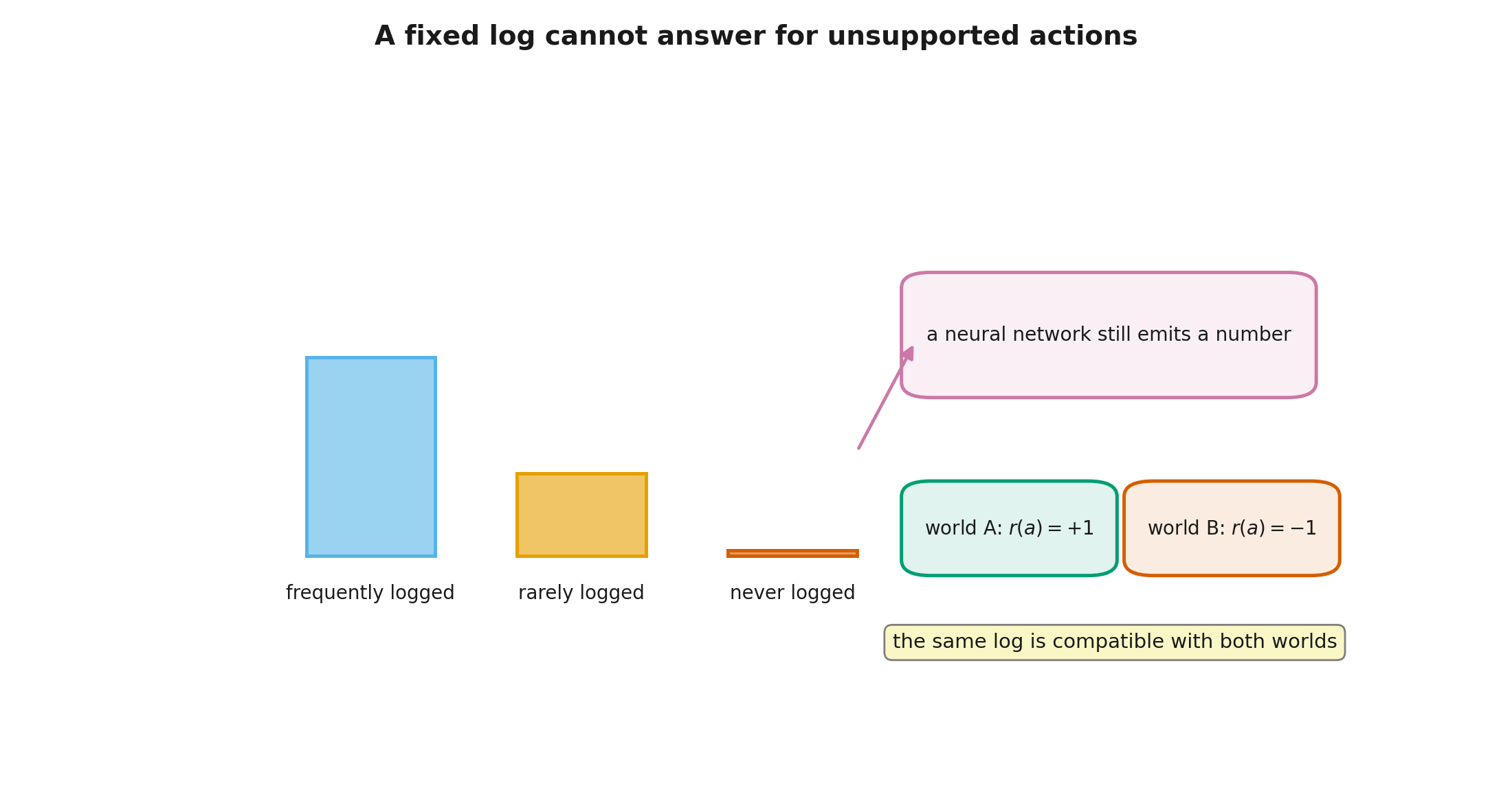
Theoretical guarantees therefore require coverage assumptions. In high-dimensional or continuous spaces, coverage is not literal state equality; it is expressed through density ratios, concentrability coefficients, representation assumptions, or related conditions.
Step 5.3.3 — Extrapolation error and a self-reinforcing loop
Suppose is trained on logged actions, but the target uses .
The maximum also considers actions that are rare or absent in the dataset. If one is accidentally overestimated, it enters the target:
The new policy then prefers this unverified action. The loop is
weak coverage → value error → selection of the error by maximization → bootstrapping → a more confident policy outside the data.
Early work often called this extrapolation error. A broader modern description includes distribution shift between the logged data and the learned policy, uncertainty in value estimates, and the policy-improvement operator itself.
Stronger generic regularization is not a universal solution. It may shrink the function but cannot reveal which unobserved action is good. The method must constrain improvement, pessimistically alter values, or train only on dataset actions.
Step 5.3.4 — Four protection mechanisms for out-of-data actions
The following is a map of mechanisms, not a ranking.
1. Restrict the action set
Batch-Constrained deep Q-learning (BCQ) learns a model of actions similar to those in the dataset and searches for improvement within that supported set. The actor is not allowed to freely exploit a Q-value for an action on which the value model was not trained.
2. Add a behavioral anchor
TD3+BC combines high estimated value with proximity to the logged action. In a simplified form,
The first term improves according to ; the second keeps the policy close to the data.
3. Lower the values of unsupported actions
Conservative Q-Learning (CQL) adds a penalty whose minimization reduces the gap between log-sum-exp values over all actions and the mean value on dataset actions. Its conservative pressure lowers unsupported actions relative to dataset actions. For discrete actions, one form is
The original analysis establishes a lower-bound property under stated conditions. A finite neural implementation with arbitrary hyperparameters does not inherit an unconditional guarantee.
4. Avoid querying out-of-data actions while learning value
Implicit Q-Learning (IQL) fits to an upper expectile of the values of dataset actions. For , it uses
Then is trained toward , and the policy is extracted by advantage-weighted BC:
usually with weight clipping.
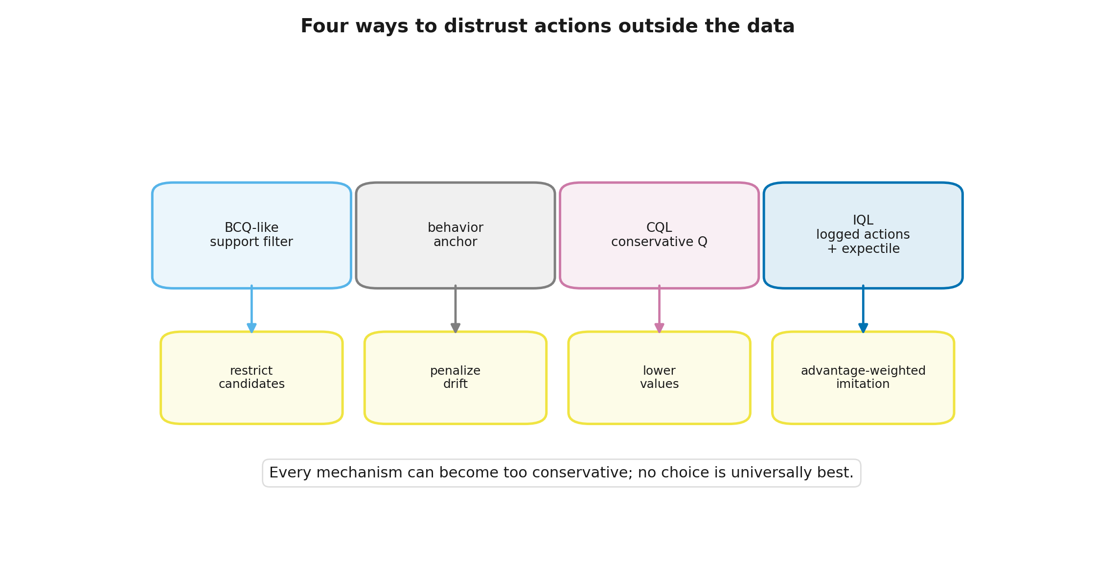
All four approaches encode the idea that improvement must respect what the data support. “Stay near the data,” however, is not one equation. Action constraints, behavior penalties, conservative value estimates, and dataset-action-only updates introduce different biases and hyperparameters.
Step 5.3.5 — Dataset quality, evaluation, and model selection
Offline-RL data quality is not determined by transition count alone. Two logs of equal size can support very different policy-improvement claims. What matters includes:
- which states and actions are covered;
- whether the log comes from one policy or a mixture;
- whether successful and failed trajectories are both represented;
- whether rewards, termination flags, and transition order are reliable;
- whether deployment dynamics match collection dynamics;
- whether evaluator training can be separated from hyperparameter selection.
Datasets for Deep Data-Driven Reinforcement Learning (D4RL) was introduced as a common collection of tasks and fixed logs for offline RL, including demonstrations, policy mixtures, and multi-task data. It was historically influential, but a D4RL result is not a certificate for another domain: dynamics, coverage geometry, reward scale, and failure cost may all differ.
Model selection is particularly difficult. A low held-out Bellman error need not imply a good policy: an estimator may fit logged actions accurately while failing on actions selected by the improved policy. One tool is fitted Q evaluation (FQE). For a fixed evaluation policy , it iteratively fits targets
There is no action maximum here: FQE evaluates a chosen policy rather than improving it. It still bootstraps from a fixed log. Weak coverage, finite data, approximation error, and policy–data shift can therefore corrupt the estimate. FQE should be paired with coverage diagnostics, multiple data splits, hyperparameter sensitivity checks, and—when safe—an independent simulator or a limited online test.
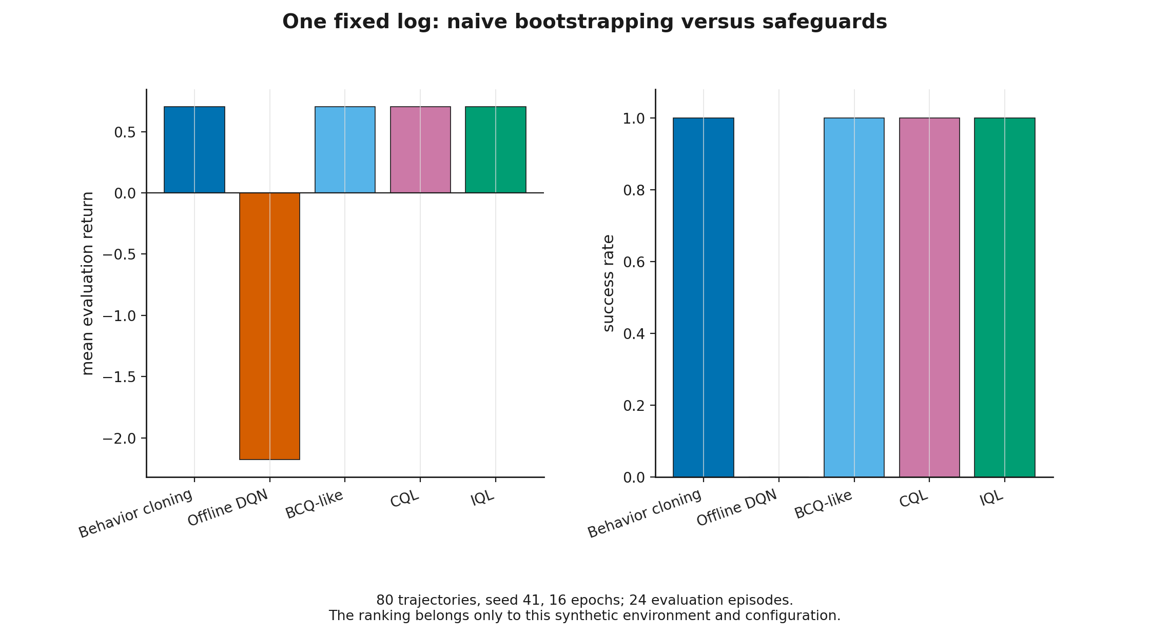
In the pinned course experiment, one log of 80 trajectories was used for BC, naive offline DQN, a BCQ-like support restriction, CQL, and IQL. With seed=41, 16 training epochs, and 24 evaluation episodes, BC, the BCQ-like method, CQL, and IQL solved every episode, whereas naive offline DQN solved none and averaged return. This is one concrete extrapolation failure in this environment, not a universal method ranking. In the same run, FQE assigned initial-state values of roughly and to BC and IQL even though direct simulator evaluation gave both policies about . On this small log, the evaluator was poorly calibrated and separated policies with the same observed performance. The full protocol is stored in data/M5_experiment_protocol.json.
Module 3 evaluated policies from one-step logs with known logging propensities. The sequential setting is harder: value errors propagate through transitions, and a new policy may visit a different part of state space. Pessimism does not remove model selection. Too little allows exploitation of error; too much collapses improvement toward mediocre behavior cloning.
Lesson 5.4. Decision Transformer: a policy as a conditional trajectory model
Lesson 5.4. Decision Transformer: a policy as a conditional trajectory model
- Put desired return into the sequence
- Updating the return condition at deployment
- How DT differs from Q-learning
- Stitching behavior fragments is not guaranteed
- Why the LLM resemblance is useful but limited
then 2 assessment steps
Step 5.4.1 — Put desired return into the sequence
Decision Transformer (DT) does not build an explicit Q-function or apply a policy gradient. It represents a trajectory as
where
is the return-to-go when .
A causal transformer predicts an action from desired return-to-go and history:
Discrete actions can use negative log-likelihood; continuous actions can use a regression loss. Optimization resembles supervised sequence modeling on fixed trajectories.
In that sense DT is conditional imitation learning: it copies actions while receiving an additional trajectory-quality condition. It can distinguish behavior in high-return trajectories from behavior in low-return ones.
Step 5.4.2 — Updating the return condition at deployment
Before an episode, choose a desired return . After action , the environment returns . For the undiscounted convention,
For the discounted recurrence
with ,
The model sees how much reward remains to be achieved, the current state, and previous actions.
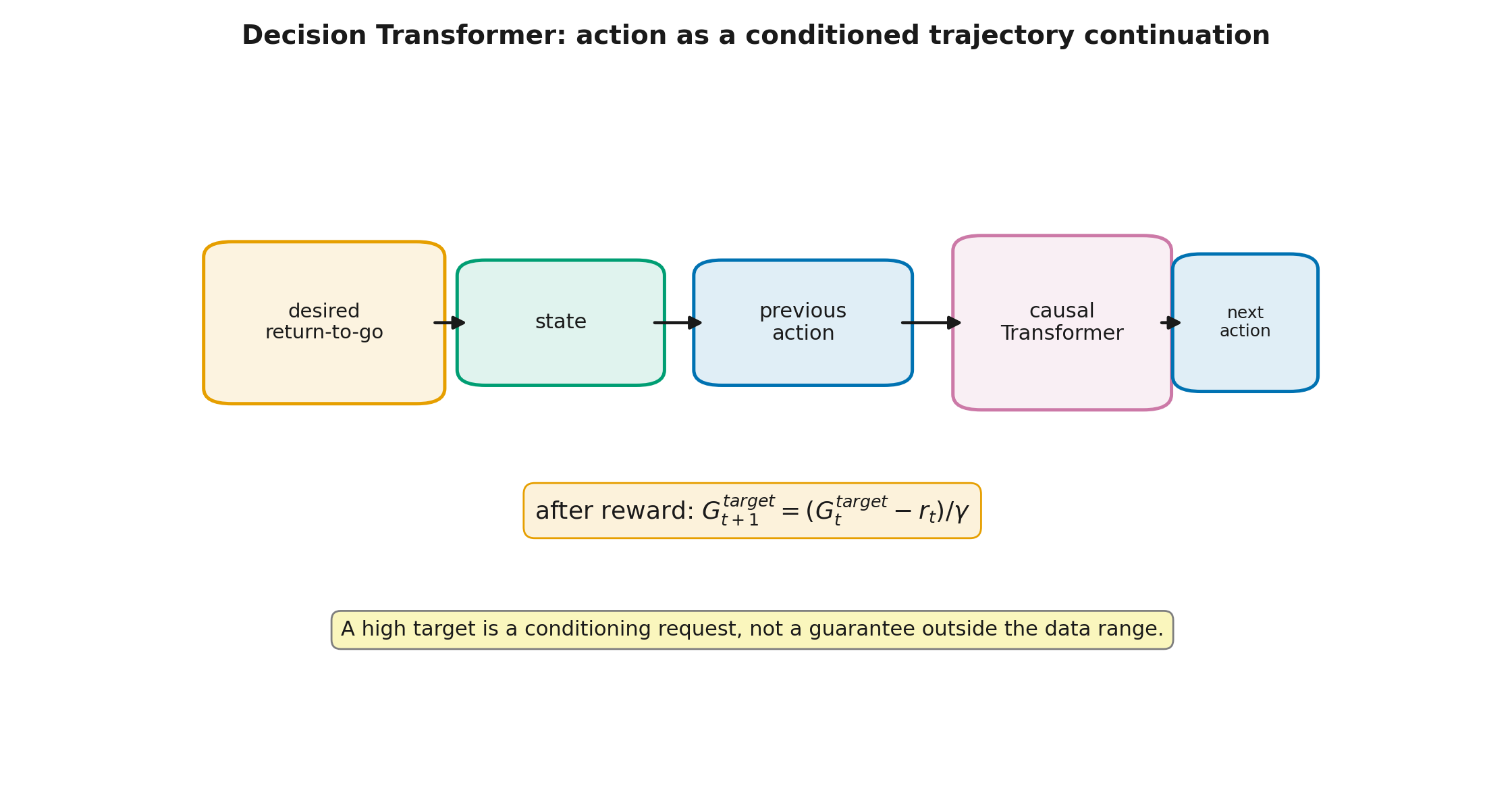
Desired return is a condition, not a promise. A target far outside the training range asks the model to extrapolate. Setting target_return=1000 does not create behavior that the model has never observed or learned to compose.
The notebook tests that distinction directly. A Decision Transformer is trained on 120 KeyDoorGrid trajectories and deployed with initial conditions , , , and . Across six evaluation episodes per condition, every setting reached the goal, while mean return stayed between about and and did not increase monotonically with the requested value. The model learned robust successful behavior, but the numerical condition did not become a calibrated return controller. This is one synthetic run, not a comparison with external DT implementations.
Step 5.4.3 — How DT differs from Q-learning
Q-learning uses a recursive relationship involving the best next action:
DT uses neither this maximum nor an explicit value function. It learns a conditional action distribution over trajectories.
This yields different strengths and failure modes.
- DT reuses standard sequence-modeling machinery and can condition on long histories.
- Q-methods explicitly exploit local dynamic recursion and can combine estimated consequences of actions.
- DT depends on coverage of relevant state–history–return combinations.
- Q-methods depend on stable bootstrapping and reliable values for candidate actions.
Neither dominates in every setting. The original DT paper reported competitive results on selected offline benchmarks; that is an empirical result for particular tasks, architectures, and datasets.
Step 5.4.4 — Stitching behavior fragments is not guaranteed
Suppose one trajectory shows how to go from to and another from to . We might hope the model will generate even though the complete trajectory is absent.
Dynamic programming makes such composition explicit through state values. A sequence model may learn it through representation generalization and attention, but its supervised objective does not supply a universal theorem of stitching for arbitrary data.
The opposite absolute claim is also wrong: DT is not fundamentally incapable of novel trajectory composition. Its ability depends on data structure, architecture, context length, scale, and optimization.
A precise summary is:
DT converts policy improvement into conditional trajectory modeling; it does not remove the coverage problem, but expresses it in the space of sequences and return conditions.
Step 5.4.5 — Why the LLM resemblance is useful but limited
DT and an LLM both use a causal transformer and autoregressive prediction. Engineering ideas such as masking, positional representations, sequence packing, context selection, and scaling therefore transfer naturally.
The analogy does not establish a direct lineage from Decision Transformer to every LLM agent, and a system prompt is not automatically a return-to-go. DT's numerical condition has a defined trajectory meaning and is updated from observed rewards. A text instruction may express a goal, style, or constraint without being a calibrated estimate of remaining return.
The useful connection is that a complex policy can be represented as a conditional sequence model. The boundary is that good conditional generation does not replace environment dynamics, data coverage, or a reward aligned with the real objective.
Lesson 5.5. A map of fixed-data LLM post-training
Lesson 5.5. A map of fixed-data LLM post-training
- First identify what was logged
- Why DPO should not simply be renamed offline RL
- ILQL: value-based offline RL for language
- A KL anchor and pessimism solve different problems
- Module summary
then 10 assessment steps
Step 5.5.1 — First identify what was logged
Algorithm choice begins with the unit of data.
| Data | Typical objective | Fresh rollouts during optimization? | What is learned |
|---|---|---|---|
| demonstrations | SFT / BC | no | demonstrator actions on demonstrator prefixes |
| transitions | classical offline RL | no | action consequences and a reward-optimizing policy |
| pairs | DPO and related methods | no | relative preference between responses |
| fresh responses with reward | PPO, RLOO, GRPO | yes | an update from current-policy rollouts |
| candidate set without weight updates | Best-of-N, search | no training | response selection at inference time |
“Offline” is sometimes used broadly for any optimization on a fixed dataset. In this course, classical offline RL means a sequential transition-and-reward problem in which action consequences are estimated and the policy is improved without further interaction.
Step 5.5.2 — Why DPO should not simply be renamed offline RL
Direct Preference Optimization (DPO) trains on fixed preference pairs and does not need to generate fresh rollouts inside each optimization step. In that broad sense it is offline policy optimization.
Its mathematical setting nevertheless differs from classical offline RL:
- data contain comparisons between whole responses rather than necessarily reward-labeled transitions;
- no Q-function is trained and no Bellman bootstrap is performed;
- the objective is derived from a KL-regularized RLHF formulation and a pairwise preference model;
- training becomes a classification-style loss involving likelihood ratios under the current and reference policies.
This course therefore calls DPO direct preference optimization on fixed pairs, not a synonym for classical offline RL. The full derivation appears in Module 8. For parallel reading, Modern LLMs, Module 14 “Learning from Feedback: RLHF, DPO, RLOO, and GRPO” (modern_llms.module_12_preference_optimization) places DPO in a modern LLM pipeline, while Information Theory for ML, Module 8 “Maximum entropy, exponential models, and KL regularization” (it_ml.module_08_maxent_kl_policy) develops the KL-regularized variational optimum.
Step 5.5.3 — ILQL: value-based offline RL for language
Implicit Language Q-Learning (ILQL) adapts IQL ideas to text generation. A prefix is a state, a next token is an action, and fixed text trajectories carry rewards or outcome scores.
The method learns and while treating out-of-data actions conservatively, then uses advantages to tilt generation toward higher-valued tokens. Unlike SFT, example quality affects more than token frequency because reward distinguishes preferred continuations. Unlike DPO, token-level value functions and sequential transitions remain central objects.
ILQL matters here as a counterexample to the claim that Q-methods cannot apply to LLMs. They can. The practical question is whether their computational cost, value-estimation stability, and reward requirements beat more direct objectives in the target setting.
The language section of the notebook builds a small but genuine offline pipeline: a fixed response log for several prompt classes, a behavior policy, token-level and heads, expectile value regression, advantage-weighted policy learning, and decoding constrained by behavior-model support. The implementation is deliberately described as ILQL-like. It reproduces the key interface, not the full architecture, scale, or every loss term of the original paper.
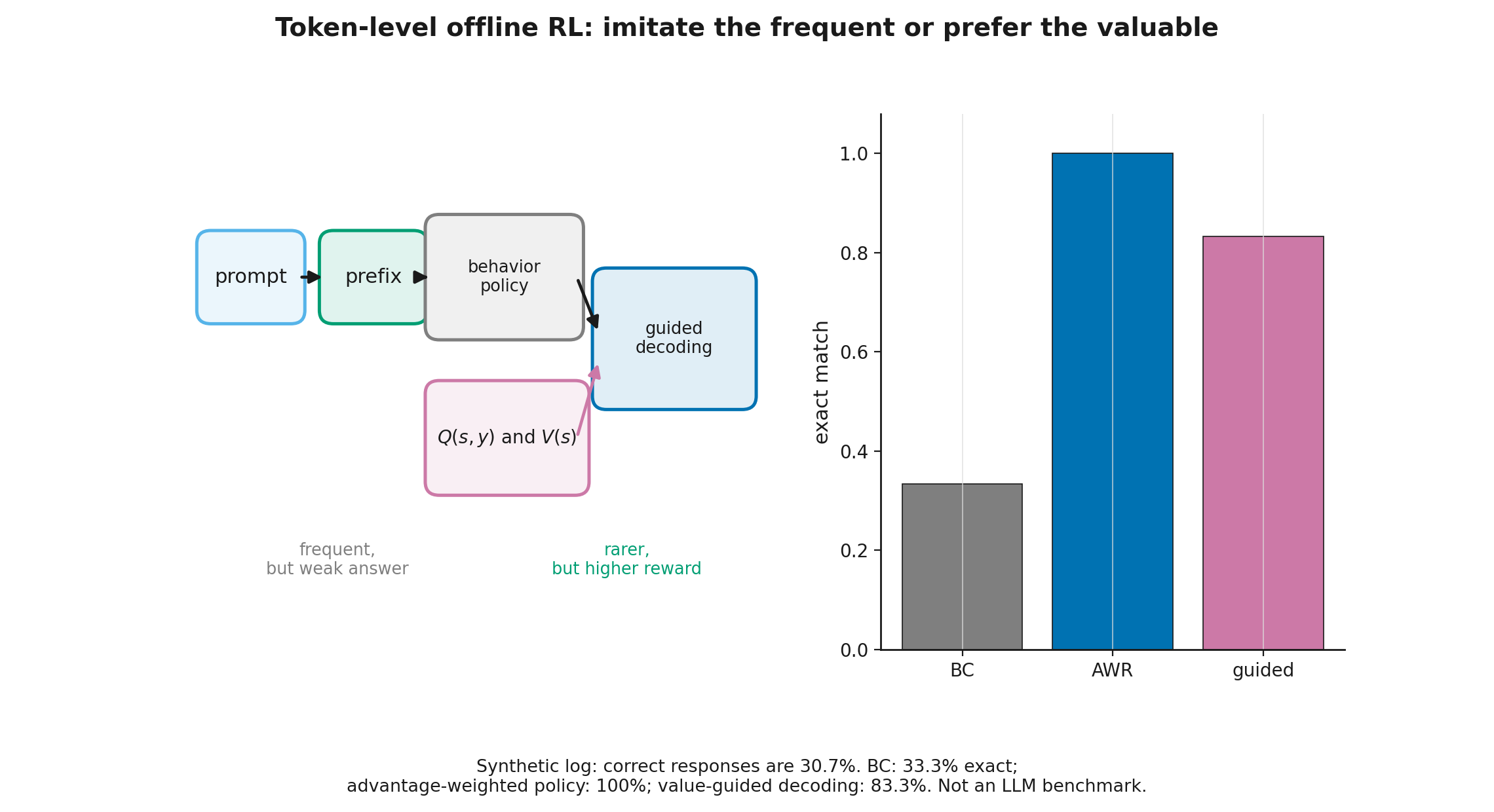
In the pinned synthetic run, exact-answer success in the logged data was about . Plain BC produced exact greedy answers, the advantage-weighted policy produced , and support-constrained value-guided decoding produced . These numbers validate mechanics under a known reward; they are not a language-quality benchmark and do not establish that an ILQL-like objective generally beats SFT.
Step 5.5.4 — A KL anchor and pessimism solve different problems
RLHF often penalizes deviation from a reference policy:
An offline-RL method may instead distrust values for poorly supported actions. Both express an engineering intuition: abrupt movement into an unknown region is risky.
Their mechanisms differ.
- KL controls a policy distribution relative to a chosen reference.
- CQL modifies value estimates.
- BCQ restricts the candidate action set.
- IQL learns values from dataset actions and extracts a policy by weighted cloning.
Small KL does not prove that the reward model is correct or that important states are covered. A conservative Q-function does not validate the reward and can become excessively pessimistic. The analogy is useful as a risk map, not as an identity of objectives.
The full variational derivation of a KL-anchored policy appears in Information Theory for ML, Module 8 “Maximum entropy, exponential models, and KL regularization” (it_ml.module_08_maxent_kl_policy). Here the important point is the interface: KL acts on a policy distribution, whereas pessimistic methods alter candidate actions, value estimates, or example weights.
Step 5.5.5 — Module summary
We can now organize the methods by data source and improvement mechanism.
- BC / SFT: copy demonstrator actions on demonstrator states.
- DAgger: add expert actions for states visited by the current policy.
- DQN: collect new transitions, reuse them, and bootstrap a Q-function.
- Offline RL: improve from fixed transitions and rewards while explicitly respecting coverage.
- Decision Transformer: predict actions as part of a trajectory conditioned on desired return-to-go.
- DPO: optimize fixed preference pairs without an explicit Q-function.
- ILQL: learn token-level values from fixed rewarded text trajectories.
The central conclusion is:
Fixing the data is not a minor implementation detail. It determines which counterfactual actions can be evaluated, which errors cannot be corrected by new experience, and which forms of regularization are meaningful.
Module 6 returns directly to the LLM policy: token log-probabilities, KL to a reference model, sampling, and sequence-level objectives.
Practice route
Practice contains 20 core tasks and 12 additional quiz questions. Worked exercise solutions expand on request. The core route covers:
- masked BC/SFT loss and an exact compounding-error calculation;
- DQN and Double-DQN targets with the correct terminal mask;
- coverage diagnostics and unsupported actions;
- CQL, expectile regression, and IQL weights;
- FQE and fixed-log model-selection risk;
- return-to-go and the Decision Transformer condition;
- token-level value guidance and the boundary of the LLM analogy.
Sources and further reading
These primary sources support the historical and algorithm-specific claims in the module. Module_5_Sources.md provides a claim-level registry, limitations, and the status of course-generated experiments.
- Ross, Gordon, and Bagnell — DAgger. Read with Step 5.1.4 for the online-learning reduction and its assumptions; the paper does not promise that one aggregation round repairs every task.
- Mnih et al. — DQN. The source for combining a deep Q-network, replay, and a target network. Atari results do not transfer automatically to KeyDoorGrid or language models.
- van Hasselt, Guez, and Silver — Double DQN. Supports separating next-action selection from evaluation and reports reduced overestimation; it does not guarantee a win on every seed.
- Fujimoto, Meger, and Precup — BCQ. Introduces support-constrained action selection and analyzes extrapolation error in fixed batches.
- Kumar et al. — CQL. Provides a conservative Q-objective and theoretical properties under stated assumptions; a chosen coefficient does not make every neural implementation an automatic lower bound.
- Kostrikov, Nair, and Levine — IQL. The source for expectile value fitting, dataset-action updates, and advantage-weighted policy extraction.
- Fu et al. — D4RL. A historically important suite of offline-RL datasets and tasks; its normalized scores are not a universal quality scale.
- Chen et al. — Decision Transformer. Introduces return-conditioned trajectory modeling. The reported benchmark results do not prove universal trajectory stitching.
- Rafailov et al. — DPO. Supports the classification-style objective on fixed preference pairs and its KL-regularized derivation; DPO is not a Bellman method.
- Snell et al. — ILQL. The source for token-level values and value-guided language generation. The course implementation is a reduced ILQL-like model, not a reproduction of every paper result.
Optional cross-course depth: Modern LLMs, Module 2 “Tokenization and Embeddings” (modern_llms.module_02_tokenization) covers special tokens and message boundaries; Modern LLMs, Module 13 “Supervised Fine-Tuning and Data Work” (modern_llms.module_11_sft) covers demonstration preparation and masking; Modern LLMs, Module 14 “Learning from Feedback: RLHF, DPO, RLOO, and GRPO” (modern_llms.module_12_preference_optimization) places fixed preferences in the LLM post-training stack; Information Theory for ML, Module 3 “Cross-Entropy and KL Divergence” (it_ml.module_03_cross_entropy_kl) develops log-likelihood and cross-entropy; Information Theory for ML, Module 8 “Maximum entropy, exponential models, and KL regularization” (it_ml.module_08_maxent_kl_policy) develops the variational logic of a KL anchor.