Module 10. Search, verification, and test-time compute
Material version: 2026.22
Factual snapshot: 2026-08-05
Language: EN
Core practice: level A — browser and CPU; level B — free Colab T4 or an optional paid API route
Structure: 5 lessons, 25 steps
Estimated time: 9–11 hours without the optional model run
Module 9 “RLVR and GRPO: verifiable rewards, group-relative estimates, and stability” (rl_llm.module_09_rlvr_grpo) changed the policy parameters using fresh rollouts. This module freezes the weights and asks a different question: how can we spend more compute on one prompt, obtain a better answer, and avoid confusing more attempts with a better selected output?
Additional compute can produce independent candidates, lengthen one trajectory, expand a search tree, or be allocated adaptively across prompts. Every design contains the same pipeline:
The generator determines which solutions are reachable. The selector determines whether a good solution can be recognized. The budget determines how many opportunities can be inspected. If any one of these components is weak, more tokens or candidates may fail to help and can even reduce deployed quality.
The practical question of the module is:
Design and validate a test-time scaling system while measuring coverage, selection quality, cost, and robustness to verifier error separately.
After completing the module, you will be able to:
- distinguish parallel, sequential, search-based, and adaptive test-time scaling;
- derive pass@N and state its assumptions;
- compute the finite-sample pass@k estimator;
- explain when self-consistency helps and when it amplifies a systematic error;
- separate the existence of a correct candidate from the ability to select it;
- analyze Best-of-N with exact and imperfect verification;
- derive the limit of a fully specified binary-verifier protocol;
- recognize proxy overoptimization as the candidate pool grows;
- distinguish outcome and process scoring and compare step aggregations;
- design beam search, best-first search, and Monte Carlo tree search without assigning them universal guarantees;
- allocate a finite budget by marginal gain;
- compare fixed training cost with higher per-query inference cost;
- run deterministic CPU experiments and prepare an optional small open-model demonstration.
Lesson 10.1. What scales at generation time
Lesson 10.1. What scales at generation time
- Frozen weights, a different answer algorithm
- Units and definitions of compute budget
- Parallel and sequential scaling are different interventions
- Search adds states and a backup rule
- Write the evaluation contract first
Step 10.1.1 — Frozen weights, a different answer algorithm
Test-time compute is extra computation performed after training for a particular prompt. The model parameters may remain fixed while the algorithm that produces the answer becomes more elaborate than one greedy decoding pass.
Four mechanisms should be kept distinct.
- Parallel compute: generate several candidates and aggregate or select one.
- Sequential compute: allow one trajectory more tokens, checks, or revisions.
- Search compute: branch, score intermediate states, and revisit promising branches.
- Adaptive compute: assign different budgets to different prompts.
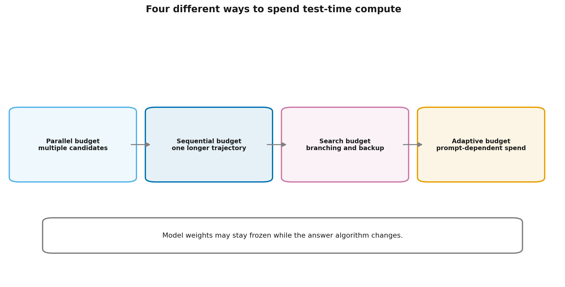
The mechanisms can be combined. A system may generate four long trajectories, score each prefix, and continue only the two most promising branches.
More compute is not an objective by itself. A valid experiment must first define quality, the measurement procedure, and the acceptable price.
Step 10.1.2 — Units and definitions of compute budget
“Four times more compute” is not a reproducible specification. A budget can mean:
- number of generated candidates;
- prompt and completion tokens;
- generator forward passes;
- verifier or judge calls;
- expanded search nodes;
- time to first token and time to final answer;
- graphics processing unit (GPU) seconds;
- peak memory;
- external API cost.
Two methods with the same candidate count can have very different cost. One may produce short answers and use cheap executable tests; another may generate long trajectories and call a separate judge model.
A minimal report records
Interactive systems also need latency quantiles rather than a mean alone. Rare multi-minute responses may be unacceptable in chat yet reasonable in batch code analysis.
Step 10.1.3 — Parallel and sequential scaling are different interventions
Parallel scaling changes sample width:
Sequential scaling changes the length or internal structure of one trajectory:
Parallel gains depend on candidate diversity and the selector. Sequential gains depend on whether the policy can use additional steps to inspect and repair its reasoning rather than repeat the same error.
Budget forcing controls reasoning length by preventing an early stop or truncating at a fixed limit. It is a useful diagnostic, not a monotonicity theorem. A longer trajectory can loop, overwrite a correct conclusion, or spend tokens on irrelevant detail.
Step 10.1.4 — Search adds states and a backup rule
Search operates on intermediate states rather than completed answers alone:
At least four components are required:
- a proposal rule;
- an intermediate-state score;
- a data structure for open candidates;
- a stopping and final-selection rule.
Search can use feedback before an answer is complete. It also creates a new failure mode: a wrong early score may prune the branch that would have produced the correct solution. Search therefore adds a controller with its own policy and errors; it is not merely “more thinking time.”
Step 10.1.5 — Write the evaluation contract first
Before the first run, fix:
- prompts and the averaging unit;
- answer extraction and canonicalization;
- generator, tokenizer, chat template, and decoding parameters;
- maximum budgets;
- aggregation or selection rule;
- verifier version;
- quality and cost metrics;
- handling of ties, abstentions, timeouts, and infrastructure errors;
- an independent set not used for tuning.
Otherwise different tasks can be compared under one budget label. pass@32 measures whether a success exists. self-consistency@32 measures a voting rule. Best-of-32 measures a particular ranker. The shared number 32 does not make the metrics interchangeable.
Extension: Modern LLMs, Module 15 “Reasoning Models and Test-Time Compute” (
modern_llms.module_13_reasoning), provides the broader history of reasoning models and product interfaces. This module owns the exact selection and cost mechanics.
Lesson 10.2. Repeated sampling and aggregation
Lesson 10.2. Repeated sampling and aggregation
- pass@N and its assumptions
- Marginal gain and diminishing returns
- The finite-sample pass@k estimator
- Self-consistency votes on canonical answers
- Canonicalization, ties, and abstention
then 4 assessment steps
Step 10.2.1 — pass@N and its assumptions
Suppose each attempt independently solves the prompt with probability . The probability that all attempts fail is , hence
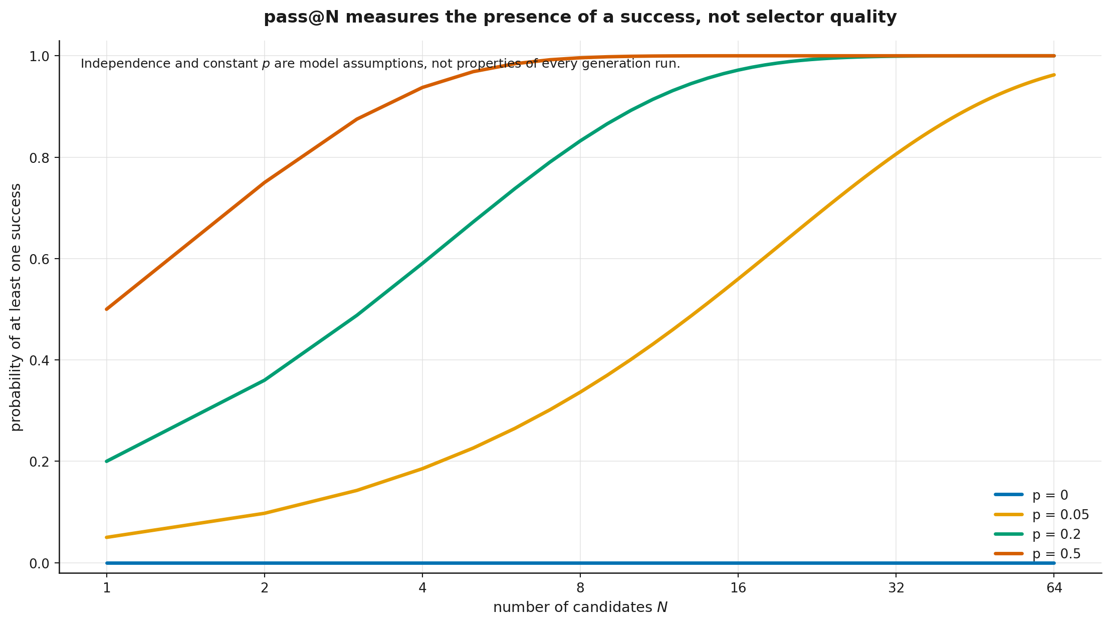
This is coverage: the probability that at least one correct candidate exists. It does not say whether the system can identify that candidate and return it to the user.
The assumptions belong next to the formula:
- attempts are conditionally independent for a fixed prompt;
- every attempt has the same success probability;
- correctness is defined before candidates are inspected;
- refers to the same decoding policy used at larger .
When generations are positively dependent and repeat one failure mode, the independence formula usually overstates the gain. “Correlation” alone does not define a universal correction, however: dependence may be clustered, driven by latent prompt difficulty, or altered by temperature. Empirical pass@k should therefore be measured from candidate groups with prompt-level records.
If , sampling cannot create support that the generator lacks. A small positive can still produce high coverage while a practical selector remains unreliable.
Step 10.2.2 — Marginal gain and diminishing returns
The gain from one additional attempt is
It is non-increasing in . For :
| Current budget | Gain from the next candidate |
|---|---|
| 0 | 0.2000 |
| 1 | 0.1600 |
| 3 | 0.1024 |
| 7 | 0.0419 |
| 15 | 0.0070 |
A large can still be worthwhile when a rare success is extremely valuable. The formula only says that decisions should be based on marginal rather than average return.
Step 10.2.3 — The finite-sample pass@k estimator
The underlying is usually unknown. A common protocol generates candidates and observes verified successes. If candidates are conceptually sampled without replacement, the probability of selecting no success is
Therefore
When , the value is one. With , , and :
This estimator belongs to a specific finite-sample protocol. Candidate counts from one decoding policy cannot be silently reinterpreted as a property of another.
Step 10.2.4 — Self-consistency votes on canonical answers
Self-consistency samples several reasoning trajectories, extracts a canonical final answer from each, and returns the most frequent answer. It votes on answers, not on the wording of the reasoning trace.
It helps when the correct canonical answer is the largest single mode while errors are dispersed across many alternatives. Under independent sampling, empirical frequencies converge to their probabilities and the correct mode wins more reliably.
Voting does not know which mode is correct. If one systematic error is more likely than the correct answer, additional votes reinforce the error.
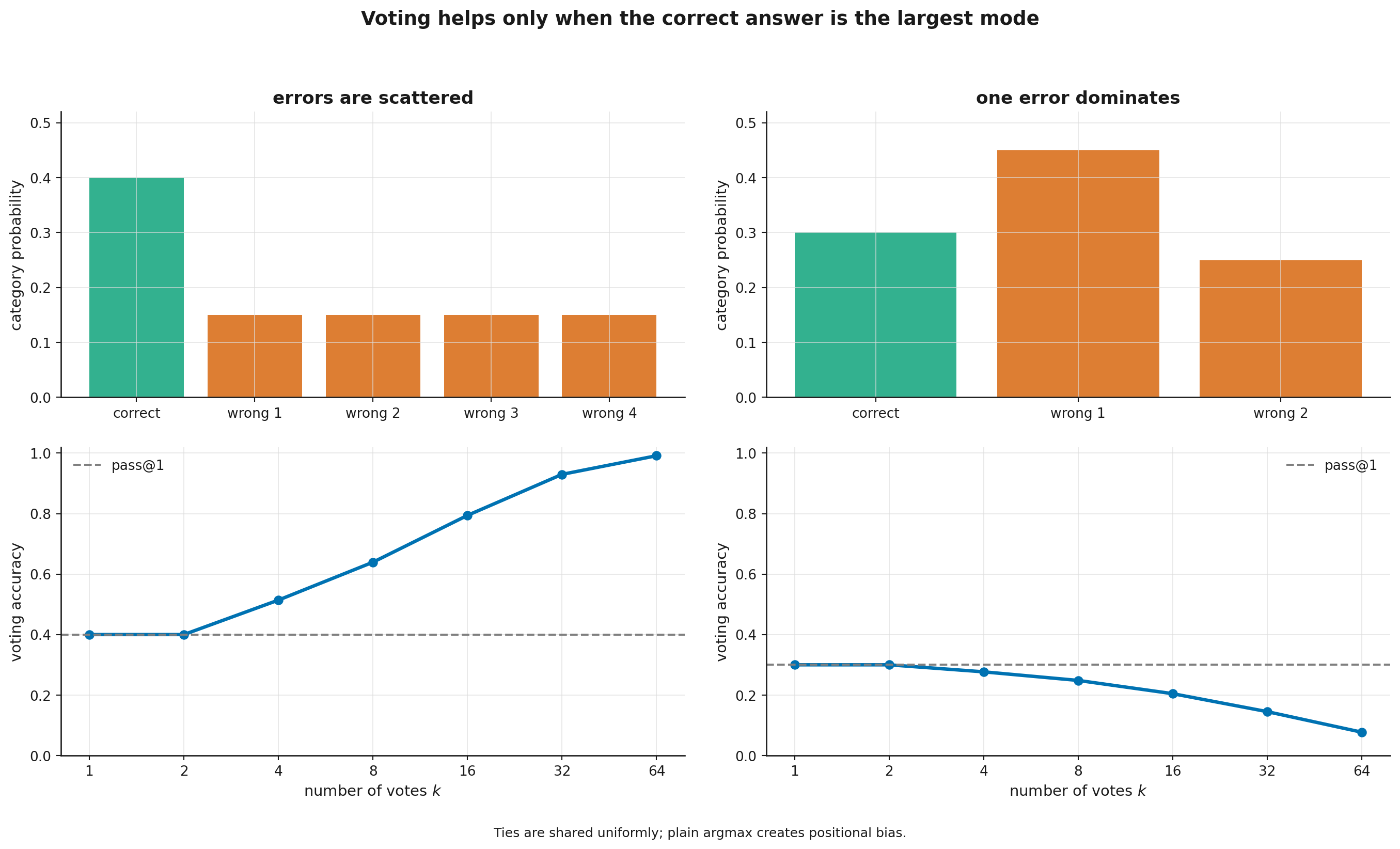
For a small number of categories, voting accuracy can be computed exactly by summing multinomial probability over all count vectors and sharing tie mass uniformly. Two teaching configurations give:
- probabilities yield accuracy about at ;
- probabilities yield accuracy about at , although
pass@64for the correct answer is essentially one.
The correct answer can be present in almost every pool while the selector almost always returns another mode.
Monte Carlo remains useful for larger answer spaces, but reports should include the trial count, random seed, and sampling uncertainty. Deterministic argmax tie-breaking is not neutral: it grants a positional advantage to the lowest index.
Step 10.2.5 — Canonicalization, ties, and abstention
Voting is not defined until the function
has been specified. Numbers can be normalized; programs can be executed against tests. Free-form text is harder: semantically equivalent answers may be phrased differently, and similar strings may contradict each other.
The protocol must define:
- what is extracted;
- how parser failure is handled;
- how ties are resolved;
- whether abstention is allowed;
- whether confidence or an external score is used;
- whether duplicate text counts as independent evidence.
A deterministic lowest-index tie rule is useful for code tests but creates a positional preference. Random tie breaking, an additional verification stage, or abstention is usually more defensible in a deployed system.
Lesson 10.3. Verifiers and Best-of-N
Lesson 10.3. Verifiers and Best-of-N
- Candidate coverage versus selection
- An exact binary-verifier model
- Ranking and the winner's error
- Five selection protocols
- Verification is part of the threat model
then 7 assessment steps
Step 10.3.1 — Candidate coverage versus selection
Best-of-N (BoN) has two stages:
- generate candidates;
- choose one with a verifier or ranker.
With perfect verification, final accuracy equals pass@N. With an imperfect selector it does not. A useful decomposition is
The first term concerns generator support and budget. The second concerns selection. Increasing may reduce the first while making the second harder because a larger pool contains more convincing false positives.
A verifier may be an exact program, tests, a reward model, a process reward model (PRM), an LLM judge, or a hybrid. These mechanisms should not be collapsed into one word without an error model.
Step 10.3.2 — An exact binary-verifier model
Consider a fully specified teaching protocol.
- A candidate is correct with probability .
- A correct candidate is accepted with true-positive rate .
- An incorrect candidate is accepted with false-positive rate .
- If any candidate is accepted, select uniformly among accepted candidates.
The single-candidate acceptance probability is
Correctness among accepted candidates is
while correctness among rejected candidates is
The second conditional probability matters when no candidate is accepted. At least two fallback protocols are possible.
Fallback to the same rejected pool
Draw a fresh independent candidate without verification
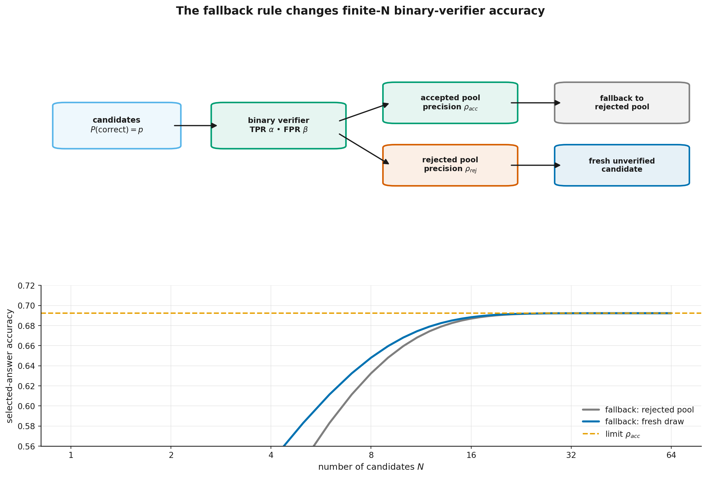
With , , and :
At :
For , the no-accept event vanishes as , so both protocols converge to . Their finite- values differ. The term is wrong when fallback selects among candidates already known to have been rejected.
Boundary. This limit belongs to binary acceptance with uniform selection among accepted candidates. It is not a universal ceiling for continuous-score ranking, pairwise tournaments, or exact verification.
Step 10.3.3 — Ranking and the winner's error
Let candidate have true utility and verifier score
BoN selects
Zero unconditional mean of alone does not imply positive mean error for the selected candidate: the joint distribution of utility and error matters. With independent, nondegenerate additive evaluator noise independent of candidate utilities, maximization favors favorable noise as well as utility. This winner's-curse mechanism can cause proxy overoptimization; without those assumptions, the sign is not guaranteed.
In the module's synthetic experiment, the proxy score rises for every larger , while the independent goal peaks at and then falls.
| Proxy score | Independent goal | |
|---|---|---|
| 1 | -0.004 | -0.075 |
| 8 | 2.005 | 0.653 |
| 32 | 2.931 | 0.723 |
| 128 | 3.670 | 0.604 |
| 512 | 4.306 | 0.253 |
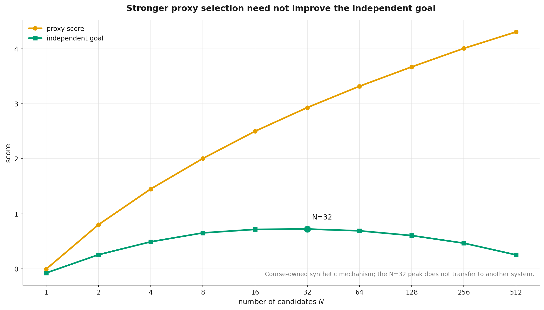
This is not a universal LLM curve. It isolates the mechanism: stronger optimization against an imperfect score requires stronger independent evaluation.
Step 10.3.4 — Five selection protocols
The same candidate pool can be processed in different ways.
| Protocol | Requirement | Main risk |
|---|---|---|
| Exact verification | executable criterion | incomplete tests or unsafe environment |
| Threshold and abstention | calibrated score | too many refusals or false accepts |
| Maximum score | comparable scale | extreme-value proxy error |
| Pairwise tournament | reliable comparisons | non-transitivity and bracket order |
| Voting | canonical answer | systematic mode |
There is no universal winner. Executable tests are usually stronger than stylistic model judgments for code, but incomplete tests may accept a solution that violates an unstated requirement. Open-ended text often lacks exact verification; calibration, abstention, candidate-order swaps, and independent rubrics then matter more.
Step 10.3.5 — Verification is part of the threat model
At large , the generator effectively searches for cases on which the verifier fails. A BoN design therefore includes:
- sandboxed code execution;
- time, memory, file-system, and network limits;
- separation of training and hidden tests;
- versioned parsers and verifier environments;
- recorded accept/reject reasons;
- false-positive audits;
- an independent control criterion;
- protection of judge instructions and rubrics.
The lesson is the same as in RLVR: reproducible reward remains a proxy. Selection pressure can be strong even when model weights never change.
Lesson 10.4. Process scores and structured search
Lesson 10.4. Process scores and structured search
- Outcome versus process feedback
- Monte Carlo labels for a prefix
- Aggregating step scores
- Beam search, best-first search, and MCTS
- Search failure modes
then 4 assessment steps
Step 10.4.1 — Outcome versus process feedback
An outcome evaluator scores a complete answer:
A PRM scores intermediate prefixes or steps:
Process feedback is useful when the final signal is sparse and search must decide which branch to continue. The semantics of depend on labeling.
- “This local step is valid” scores a local property.
- “This prefix often leads to success” estimates success under a particular continuation policy.
- “An expert prefers this prefix” defines another object.
Calling all three a state value without qualification is incorrect.
Step 10.4.2 — Monte Carlo labels for a prefix
From prefix , generate independent continuations under policy . Let indicate final success. Then
estimates
This connects directly to Monte Carlo evaluation in Module 2 “State, Value, and Bellman Equations” (rl_llm.module_02_values_bellman). It also fixes the scope: the label depends on continuation policy , decoding, budget, and final criterion. It may become stale when the policy changes.
A zero label from a small does not prove impossibility. If the true success probability is , observing no success in ten continuations has probability
Even six successes out of eight give point estimate but a wide approximate 95% Wilson interval, about . For a process model, two nearby raw means may therefore fail to define a reliable ordering.
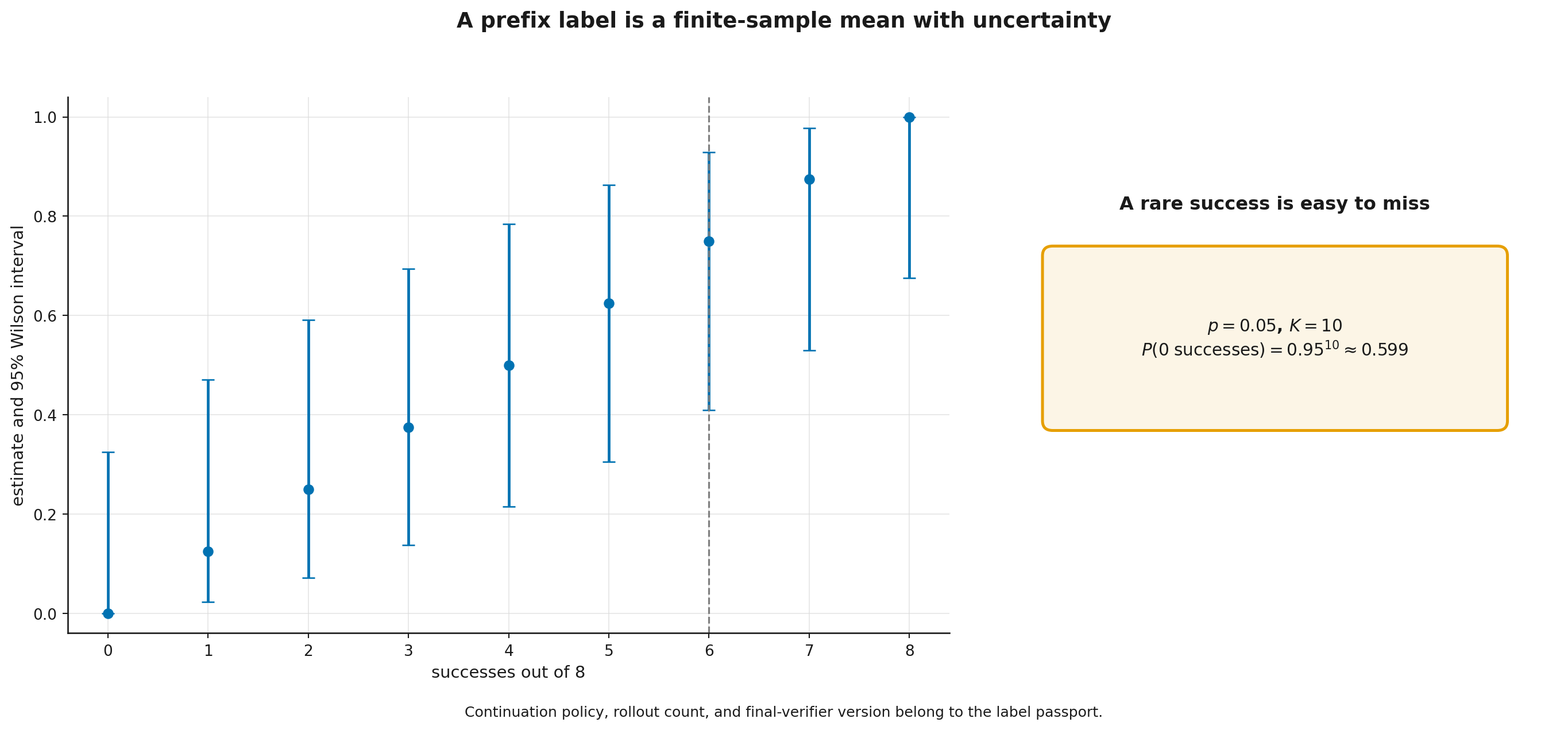
A label passport should record continuation count, policy and decoding parameters, final-verifier version, and an uncertainty or smoothing rule. Equal weighting of raw means also needs justification when prefixes receive different numbers of continuations.
Step 10.4.3 — Aggregating step scores
Given , common rules include
For :
| Rule | Value | Emphasis |
|---|---|---|
| minimum | 0.3000 | weakest step |
| mean | 0.7875 | average level |
| product | 0.2572 | joint chain under strong assumptions |
| last | 0.9500 | final prefix only |
A product contains an implicit length dependence. A constant score gives and . This can be meaningful when scores are compatible conditional probabilities in one factorization. Otherwise it is a hidden length penalty.
The minimum is sensitive to one noisy dip, the mean can conceal a fatal step, and the last score ignores early violations. Aggregation must follow label semantics rather than library habit.
Step 10.4.4 — Beam search, best-first search, and MCTS
Beam search keeps the best current prefixes, expands them, and prunes back to . It is simple and vectorizable, but early pruning is irreversible.
Best-first search keeps a global frontier and expands the currently highest-scoring state. It supports uneven depth but requires scores that are comparable across depths.
Monte Carlo tree search (MCTS) typically alternates selection, expansion, evaluation or simulation, and backup to ancestors.
Classical UCT (Upper Confidence bounds applied to Trees) assigns a visited child an index of the form
where is the child's mean return, is the parent's visit count, is the child's count, and controls exploration. Unvisited children normally receive a separate expansion priority.
The relation to UCB in Module 3 “Bandits, exploration, and one-step decisions” (rl_llm.module_03_bandits) is conceptually useful, but it does not import guarantees automatically. Text trees have enormous branching, string-distinct semantic duplicates, biased evaluation, and variable-length actions. Modern systems often use priors and PUCT-like variants; the exact formula and cost unit should be named.
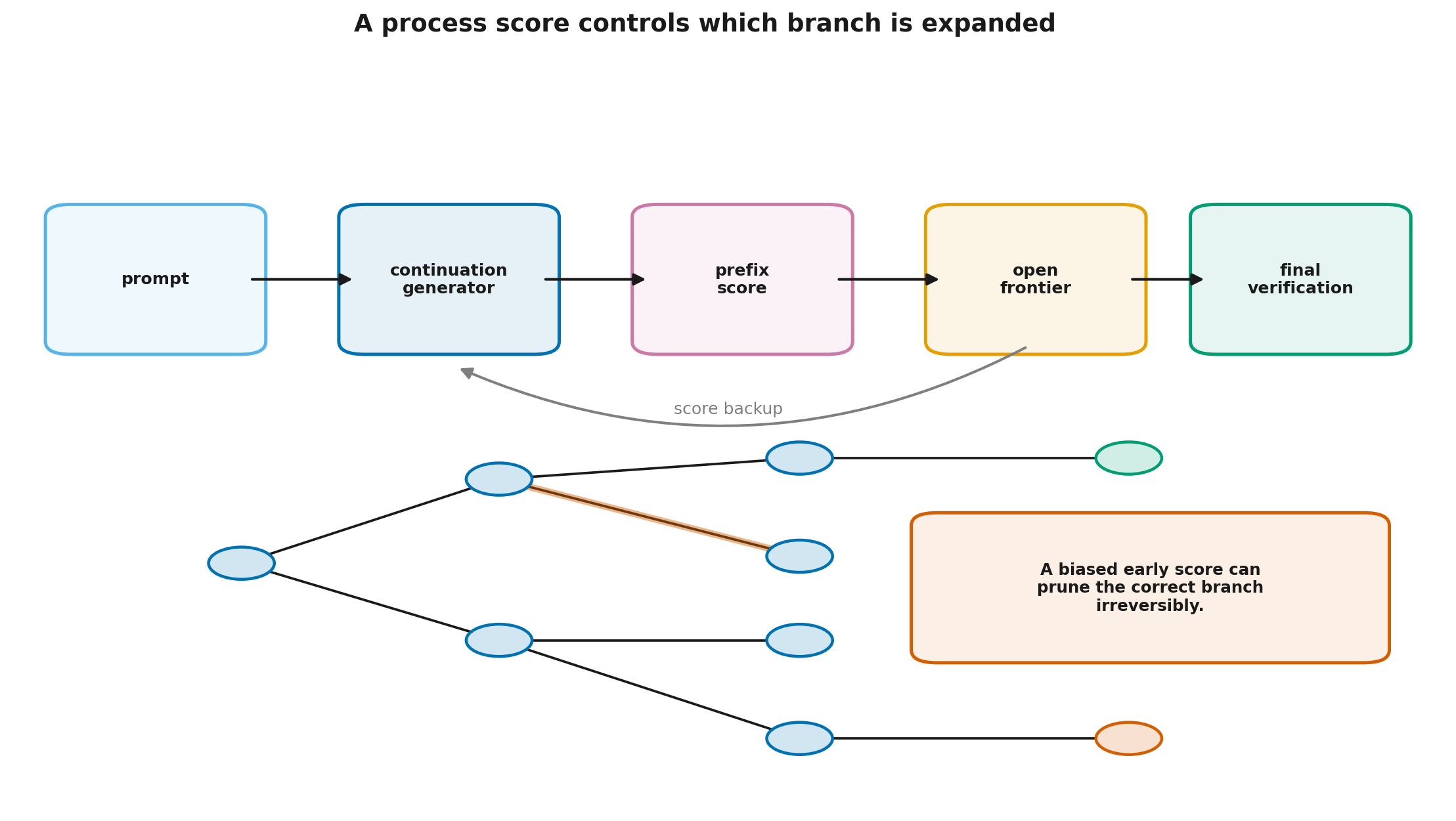
Step 10.4.5 — Search failure modes
Structured search can lose to repeated sampling when:
- prefix scoring is worse than final verification;
- the correct branch looks weak early;
- proposals lack diversity;
- width and depth are mismatched to the task;
- scores across depths are incomparable;
- the local verifier can be exploited;
- tree-management overhead consumes the gain;
- several branches are paraphrases of one error.
The notebook includes a small “reasoning maze.” A frozen proposal policy chooses the next step, an exact goal check supplies outcome verification, and a process score guides beam, best-first, and PUCT-like search. One proposal call is one budget unit.
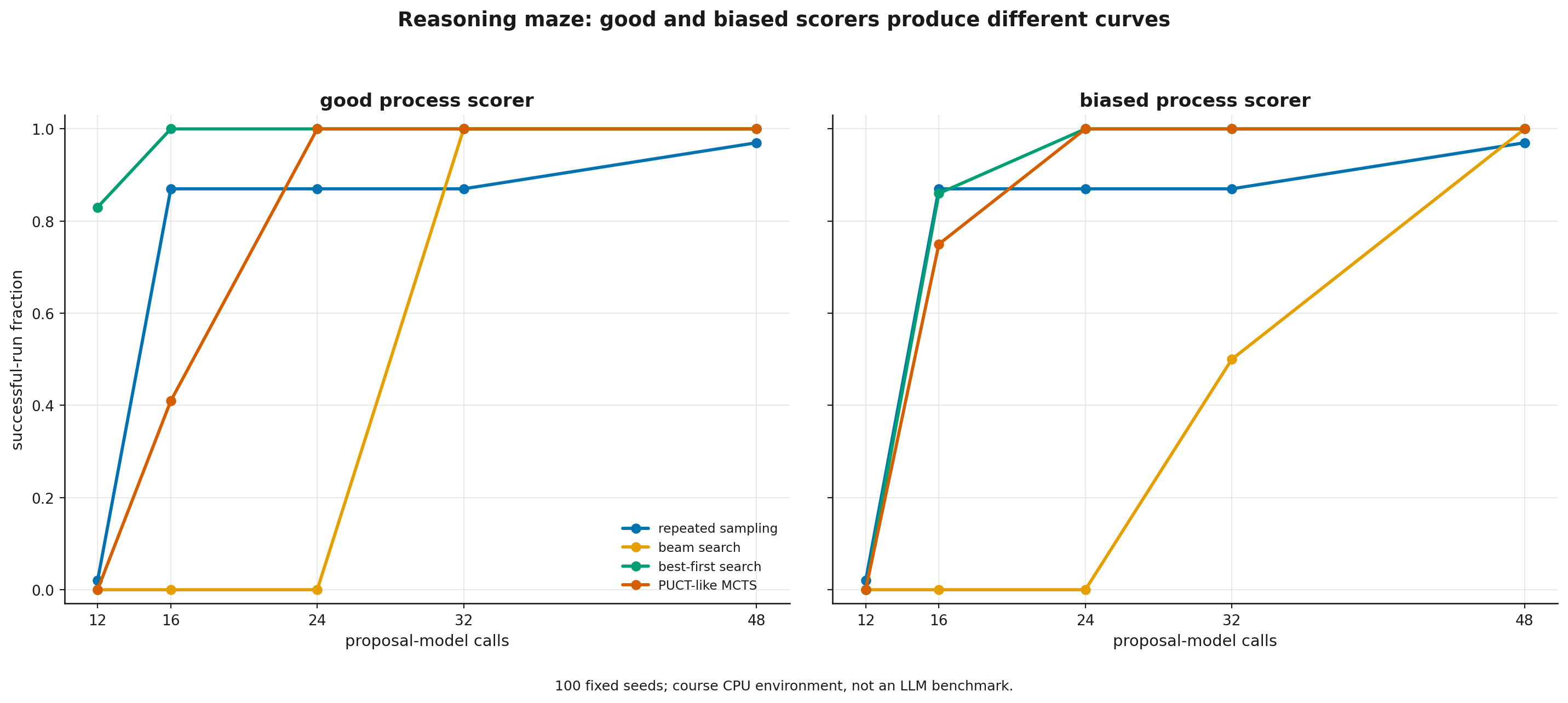
In the fixed synthetic protocol, a good geometric scorer lets best-first search find the route earlier than repeated sampling. A biased scorer delays best-first search and worsens early beam pruning. With enough budget, the small environment becomes easy for almost every method. These are course-code results, not an LLM benchmark or a theorem that one search algorithm dominates.
Every comparison should therefore include cost-matched simple baselines: one answer, repeated sampling, self-consistency, and BoN. Search is justified by a better independent quality–cost frontier, not by architectural complexity. Reports should also retain tree coverage, proposal calls, scorer version, and examples of incorrectly pruned branches.
Lesson 10.5. Adaptive budgets and economics
Lesson 10.5. Adaptive budgets and economics
- An objective with compute cost
- Marginal gain and adaptive allocation
- Stopping rules
- Train better or infer more expensively
- Release protocol for a search system
then 7 assessment steps
Step 10.5.1 — An objective with compute cost
One formulation is
where is a generation mode, expected quality, cost, and converts cost into utility units.
A constrained form is
Both force the cost definition to be explicit. GPU-seconds may dominate batch processing; end-to-end latency may dominate chat. Paid judge calls belong in just like generator tokens.
The non-dominated operating points form a Pareto frontier. Selecting one point is a product decision, not an intrinsic property of an algorithm.
Step 10.5.2 — Marginal gain and adaptive allocation
Suppose prompt has independent single-attempt success probability . Its coverage after attempts is
with next-sample gain
These gains are non-increasing. Under this exact model, an integer budget can be allocated greedily by repeatedly assigning the next sample to the prompt with the largest current . An exchange argument shows this is optimal among allocations that satisfy the declared per-prompt minimum.
That minimum is a separate product decision, not a consequence of the formula. allocate_budget_greedy defaults to minimum_per_prompt = 1: every prompt receives at least one attempt and the remainder is allocated greedily. It is a reasonable service guarantee — no prompt left without an answer — but it lowers achievable coverage.
For
and a total budget of 16, uniform allocation yields mean coverage . The greedy rule with minimum_per_prompt = 1 produces
and mean coverage . Without the floor () the same rule produces
and mean coverage — the global optimum, confirmed by exhaustive search. The gap of is the price of the "at least one attempt per prompt" guarantee: a near-hopeless prompt with consumes an attempt worth more on the prompt with .
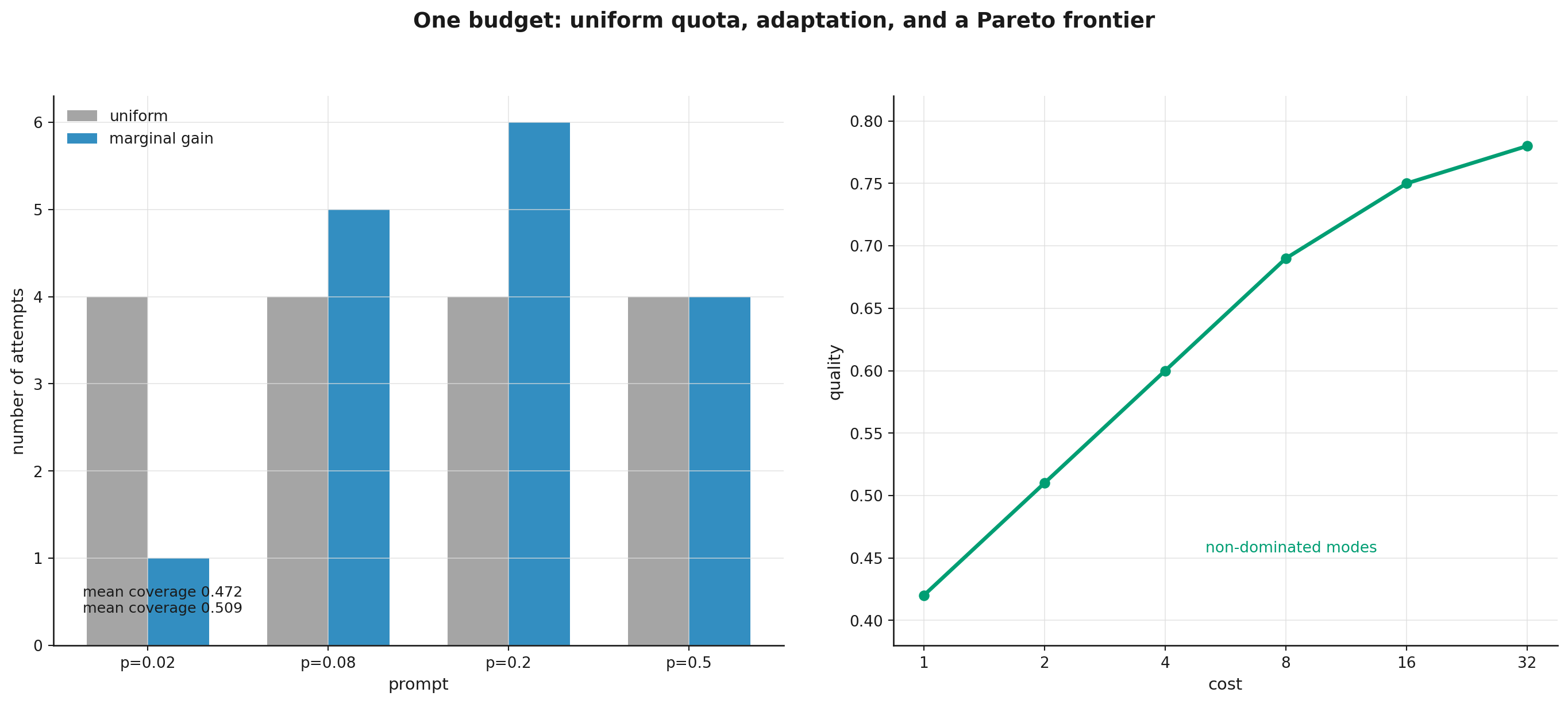
This is exact for known and independent attempts. Real systems must estimate difficulty, and the difficulty estimator can itself be miscalibrated. Adaptivity adds another model that requires validation.
Step 10.5.3 — Stopping rules
A system may stop when:
- exact verification succeeds;
- a voting lead is mathematically irreversible under the remaining budget;
- marginal gain is small;
- several independent evaluators agree;
- time, token, or monetary budget is exhausted;
- proxy-overoptimization risk becomes unacceptable;
- uncertainty remains high enough to justify abstention.
For self-consistency, an irreversible lead can save samples relative to a fixed maximum, but it does not repair a systematically wrong leader.
For continuous-score BoN there is no universal “good enough” score. A calibrated probability of success and the cost of another candidate are more useful than the raw maximum score.
Step 10.5.4 — Train better or infer more expensively
Suppose additional training costs and reduces per-query cost from to at acceptable quality. The cost-only break-even volume is
With , , and :
If the new system is not cheaper per query, there is no cost-only break-even point. Even a finite point is insufficient: quality, latency, risk, and system lifetime must also be compared.
Expensive inference is often faster to deploy for small or changing traffic. At large stable volume, training, distillation, or a specialized ranker can amortize a fixed cost.
Step 10.5.5 — Release protocol for a search system
Record four layers before publication.
Generator
- model and tokenizer versions;
- chat template;
- temperature, top-k, top-p, and length limits;
- seed and candidate count;
- sequential budget rules.
Selection and search
- answer canonicalizer;
- verifier or PRM;
- step aggregation;
- search algorithm and hyperparameters;
- ties, abstention, and stopping.
Cost
- generator and judge tokens;
- expanded nodes;
- latency and GPU-seconds;
- API price;
- retries and environment failures.
Independent quality
- pass@1 and pass@k;
- accuracy of the actually selected answer;
- calibration and abstention rate;
- quality by difficulty slice;
- robustness to rephrasing and verifier changes;
- audit cases where proxy and independent goal disagree.
This module stayed within one prompt and a controlled reasoning tree. Module 11 “RL for LLM agents: tools, environments, and long trajectories” (rl_llm.module_11_agentic_rl) adds external state, tools, hidden variables, and multi-turn episodes. Module 12 “RL infrastructure for LLMs: memory, rollouts, and asynchrony” (rl_llm.module_12_infrastructure) covers distributed trajectory collection and policy versioning. Module 13 “Evaluating RL systems for LLMs: statistics, reward hacking, and safety” (rl_llm.module_13_evaluation) develops independent evaluation and metric gaming in depth.
Sources and reading route
The following primary sources support the module’s main external claims. Course-derived formulas, exact calculations, and synthetic results are documented in the English claim and source registry.
- Wang et al., Self-Consistency Improves Chain of Thought Reasoning in Language Models — the original multiple-trajectory and answer-aggregation protocol. It reports gains on selected tasks, not a guarantee under a dominant systematic error.
- Chen et al., Evaluating Large Language Models Trained on Code — HumanEval and the finite-sample
pass@kestimator. The expression belongs to a defined sampling and verification protocol. - Brown et al., Large Language Monkeys: Scaling Inference Compute with Repeated Sampling — repeated-sampling scale and the distinction between candidate coverage and recognizing a success.
- Lightman et al., Let’s Verify Step by Step — process supervision, PRM800K, and the paper’s selection experiments. It does not make every process score a calibrated value function.
- Yao et al., Tree of Thoughts: Deliberate Problem Solving with Large Language Models — branching over intermediate states, evaluation, lookahead, and backtracking.
- Kocsis and Szepesvári, Bandit Based Monte-Carlo Planning — classical UCT. Its guarantees do not transfer automatically to language trees with learned evaluators.
- Snell et al., Scaling LLM Test-Time Compute Optimally can be More Effective than Scaling Model Parameters — prompt-dependent test-time scaling and adaptive compute in the studied setup.
- Muennighoff et al., s1: Simple test-time scaling —
budget forcingthrough forced continuation or early termination; an empirical method, not a theorem that longer reasoning is always better. - Gao, Schulman, Hilton, Scaling Laws for Reward Model Overoptimization — reward-model overoptimization under stronger selection pressure, including Best-of-N.
- Official Transformers generation documentation and the Qwen3-0.6B model card — used only by the optional engineering branch; the core notebook runs offline on CPU.
Cross-references
- Module 2 “State, Value, and Bellman Equations” (
rl_llm.module_02_values_bellman): Monte Carlo prefix values and value backup along trajectories. - Module 3 “Bandits, exploration, and one-step decisions” (
rl_llm.module_03_bandits): UCB, exploration, and constrained budget allocation. - Module 6 “The LLM as a policy: tokens, log-probabilities, and KL” (
rl_llm.module_06_llm_policy): the actual generation distribution and decoding parameters. - Module 7 “Reward models and preference data” (
rl_llm.module_07_reward_models): calibration, winner's error, and proxy overoptimization. - Module 9 “RLVR and GRPO: verifiable rewards, group-relative estimates, and stability” (
rl_llm.module_09_rlvr_grpo): verifier contracts, process feedback, and rollout cost. - Information Theory for ML, Module 2 “Entropy” (
it_ml.module_02_entropy): candidate-distribution entropy and limits of diversity metrics. - Information Theory for ML, Module 3 “Cross-Entropy and KL Divergence” (
it_ml.module_03_cross_entropy_kl): logarithmic scores, KL, and distribution comparison. - Modern LLMs, Module 10 “KV Caches and Efficient Inference” (
modern_llms.module_09_inference): engineering decoding modes, latency, and serving. - Modern LLMs, Module 15 “Reasoning Models and Test-Time Compute” (
modern_llms.module_13_reasoning): the broader landscape of reasoning models and current interfaces.
Key takeaways
- pass@N measures the presence of a success under explicit assumptions, not selector quality.
- Self-consistency removes dispersed error and amplifies the most likely systematic mode.
- An imperfect verifier defines its own quality frontier and can be overoptimized at large .
- A PRM is useful only after its labels and step aggregation have been defined.
- Search enables revisiting decisions but adds early pruning and new proxy objectives.
- Budgets should be allocated by marginal gain and measured in tokens, latency, compute, and money.
- Training versus expensive inference depends on traffic, lifetime, quality, and risk—not on one per-query price alone.