Module 1. Introduction: Reinforcement Learning for LLMs
Content version: 2026.18
Fact snapshot: 2026-07-16
Language: EN
Core practice: Tier A — browser and central processing unit
Structure: 4 lessons, 19 steps
Estimated time: 5–7 hours, excluding optional exercises
This course applies RL to LLMs. A prior RL course is not required. You should be comfortable with Python, basic PyTorch, probability, gradient optimization, and the Transformer architecture.
Two reading routes. If RL is new to you, read Lesson 1.1 in order; it introduces the complete minimum vocabulary. If you have studied classical RL, skim §§1.1.1–1.1.3 and spend more time on §§1.1.4–1.1.6, where familiar notation is connected to LLMs and the boundary between RL and neighboring post-training methods is made explicit.
Module goals. After completing the module, you should be able to:
- describe the agent → action → environment → observation-and-reward loop;
- distinguish states, observations, actions, rewards, episodes, trajectories, and policies;
- explain the exact sense in which an LLM is a stochastic policy;
- compute a return and read in words;
- choose among a one-response model, a token-level Markov model, and a multi-step agentic formulation;
- distinguish learning from demonstrations, direct preference optimization, online policy optimization, and candidate selection without parameter updates;
- complete four reproducible Tier-A exercises: return, stable softmax, entropy, and Monte Carlo policy evaluation.
Practice route. Graded tasks, worked solutions revealed after an attempt, and executable practice follow the lecture. The explanation remains self-contained.
Lesson 1.1. The Minimum Language of Reinforcement Learning
Lesson 1.1. The Minimum Language of Reinforcement Learning
- What RL is: one loop before a catalog of algorithms
- Agent, environment, state, action, and reward
- Policy: a rule for choosing actions
- An LLM as a policy: the exact correspondence and its boundary
- Reward, return, discounting, and the RL objective
- Why RL is not merely “learning without a correct answer”
then 9 assessment steps
Step 1.1.1 — What RL is: one loop before a catalog of algorithms
We will begin with the problem, not with algorithm names or Bellman equations.
In supervised learning, an example usually comes with a target: an image class, a translation, or a spam label. In self-supervised learning, the target is extracted from the data itself. In next-token prediction, the correct continuation is already present in the corpus.
In RL, the central object is an agent that chooses actions in an environment and receives a reward, a scalar feedback signal about the outcome. The agent does not merely predict a target recorded in advance: its decisions affect what happens next and which data it will observe.
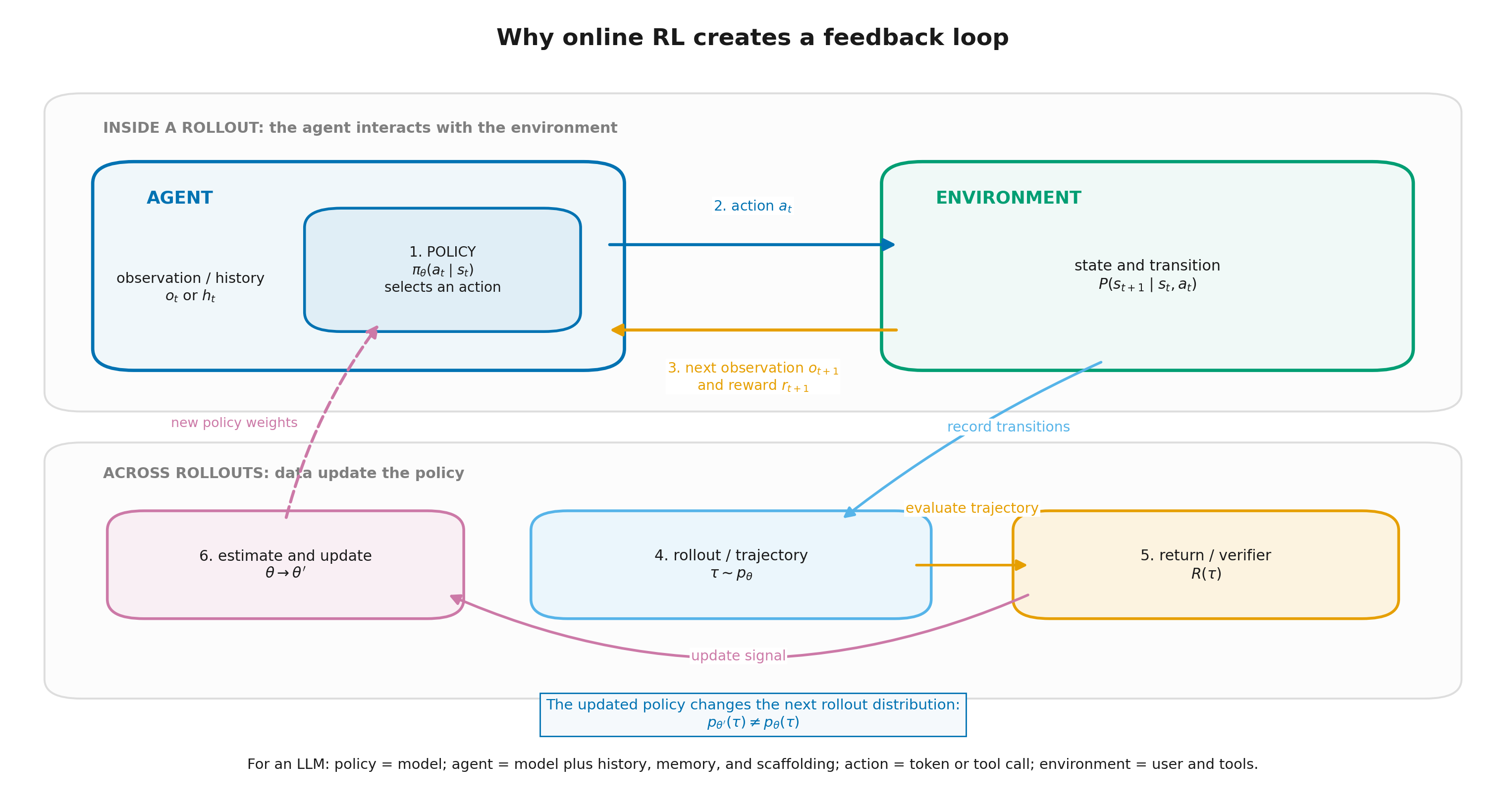
The figure separates two connected time scales. The upper part is interaction inside one rollout. The lower part is learning across rollouts.
- The agent receives a state or observation. The agent contains a policy , the rule used to select actions.
- The policy selects an action and sends it to the environment.
- The environment changes its state and returns the next observation and a local reward .
- A sequence of such transitions forms a rollout, or trajectory .
- The trajectory is evaluated by a return, an executable verifier, a reward model, or an environment outcome.
- The learning algorithm uses the data and feedback to update . The updated policy changes the distribution of future trajectories, so need not equal .
This is why online RL is a feedback loop: the policy changes the data, the data changes the policy, and the update changes future data. Agent and policy are not synonyms: the policy is the action-selection mechanism inside the agent, while the environment is everything that receives actions and returns their consequences.
Two short examples make the pattern concrete.
- A corridor. The agent occupies a cell, chooses left or right, and receives if it reaches the right terminal state.
- An LLM. The model sees a prompt and the generated prefix, chooses the next token or a larger action, and a checking system scores the outcome.
For a first pass, keep one sentence:
RL studies how to choose actions from feedback so that the expected outcome of a sequence of decisions improves.
We will sharpen this definition later. In particular, “there is no correct answer in RL” is a useful first intuition but not a sufficient formal boundary.
Step 1.1.2 — Agent, environment, state, action, and reward
Let us fix the basic vocabulary. At time :
- the agent is the decision-making system;
- the environment is everything that responds to the agent's actions and determines their consequences;
- the state describes the situation well enough to model the next transition;
- the observation is the information actually available to the agent and may be incomplete;
- the action is the agent's choice from an action space ;
- the reward is a local scalar signal following an action;
- the transition describes environment dynamics;
- an episode runs from an initial condition to a terminal condition or time limit;
- a trajectory records an episode.
When the chosen state contains all information needed to determine the distribution of the next state and reward, the model is a Markov decision process (MDP). “Markov” does not mean that the world has no memory; it means that all relevant memory has been included in the state.
A finite MDP is often written as
where is the state space, the action space, the dynamics, the reward rule, the initial-state distribution, and the discount factor. You do not need to memorize the tuple separately; every component has already been introduced in words.
The same concepts can be placed side by side in a toy environment and in an LLM.
| Concept | Corridor | Token generation by an LLM |
|---|---|---|
| Agent | movement rule | Transformer with its current weights |
| Environment | cells and terminal states | token append, length limit, evaluator |
| State | cell index | prompt + generated prefix |
| Action | left / right | next token |
| Reward | at the right terminal | for example, whether tests pass or how the response is scored |
| Episode | path to a terminal | generation until an end-of-sequence token or a length limit |
An end-of-sequence token (EOS) terminates a response in much the same way that a terminal cell ends a corridor episode.
Do not confuse a reward with the environment. A learned reward model, a unit-test suite, a mathematical verifier, or a user may compute the reward. The environment also includes transitions, constraints, hidden tool state, and everything else that determines the next step.
Step 1.1.3 — Policy: a rule for choosing actions
A policy is the rule by which an agent chooses an action.
A deterministic policy returns one action:
A stochastic policy defines a probability distribution over actions:
In deep RL, the policy is usually parameterized by a neural network:
where denotes trainable weights. The network first produces action scores, those scores are converted into a distribution, and a concrete action is then selected from that distribution.
Three objects should remain separate.
- The policy is the entire distribution .
- The action is one concrete sample from that distribution.
- The reward is a later assessment of the outcome; it is not a policy probability.
Stochasticity is not present merely for “randomness.” It permits exploration, produces diverse experience, and allows relative action probabilities to change smoothly. At inference time a policy may be made nearly deterministic, but collapsing it too early during training can remove useful alternatives.
Step 1.1.4 — An LLM as a policy: the exact correspondence and its boundary
We can now build the main bridge of the course.
Let be a prompt and the generated prefix. In a token-level formulation,
The Transformer produces logits and defines a next-token distribution:
Thus an LLM really is : the context is the state, the next token is the action, and the Transformer weights are the policy parameters. Within this token-level abstraction, the correspondence is mathematical rather than metaphorical.
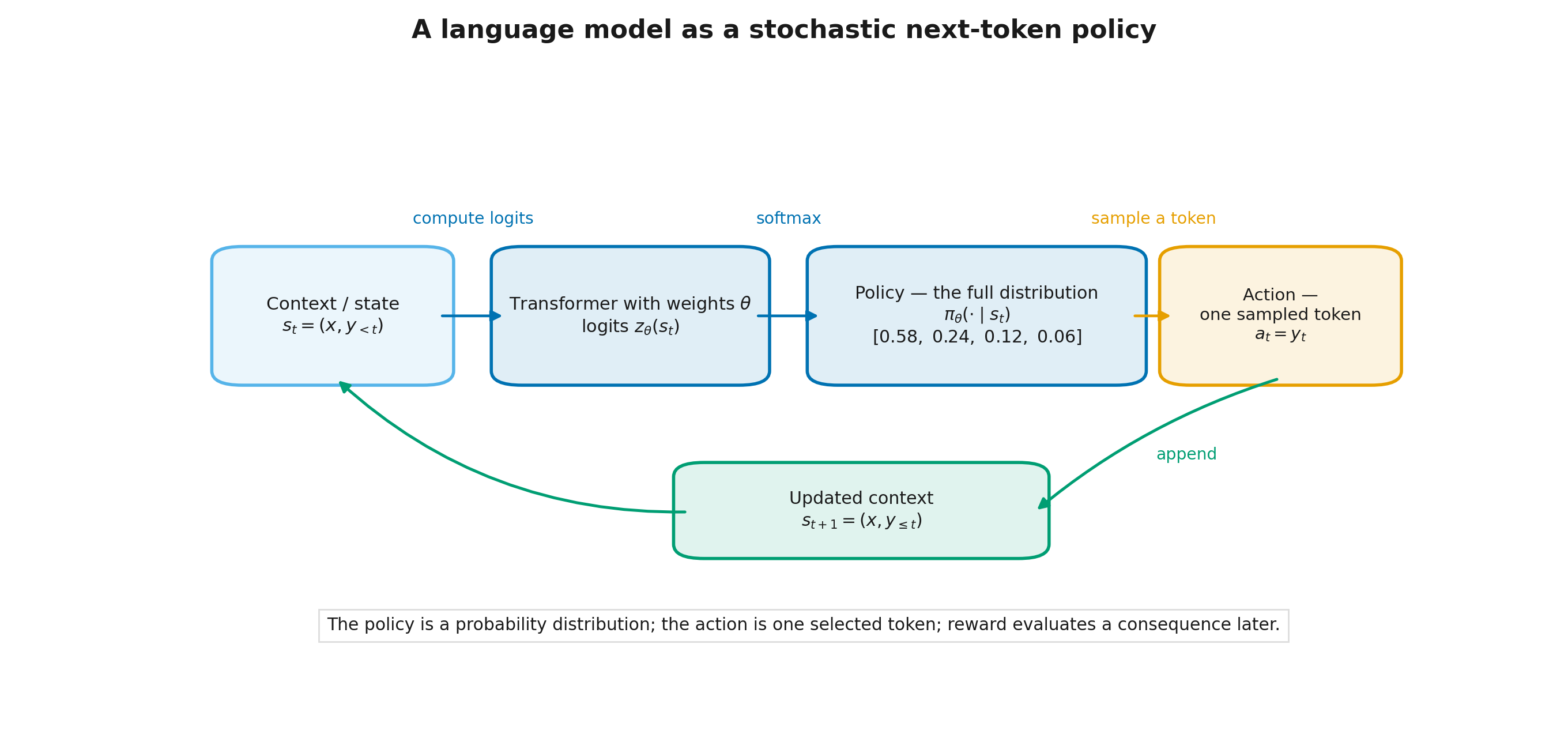
The probability of a complete response factorizes autoregressively:
and the log-probability converts the product into a sum:
These two equations will reappear in policy-gradient methods and in regularization by the Kullback–Leibler divergence (KL). We will name the concrete preference and group-relative algorithms after the basic formulation is complete.
Two boundaries matter.
- Calling an LLM a policy describes how it chooses actions; it does not claim that its weights were necessarily trained with RL. A pretrained model already defines a policy even though it was trained by next-token prediction.
- In a deployed system, the LLM is usually a policy or a policy component, not the whole environment. External tools, files, browsers, users, and verifiers have their own state and dynamics.
“An LLM is a policy” is therefore exact once the state and action have been specified.
Step 1.1.5 — Reward, return, discounting, and the RL objective
A reward belongs to one transition. The return is the accumulated future reward from time :
Here is the discount factor. It may serve several roles:
- assign lower weight to more distant consequences;
- control an effective planning horizon;
- make an infinite-horizon sum converge.
Finite-response LLM training often uses : EOS or a maximum length already bounds the episode, and the final score applies to the response as a whole. This is not universal. Delay, time cost, and interruption risk can make meaningful in long agentic tasks.
For rewards and ,
The RL objective fits in one line:
Read it in words: we seek policy parameters under which trajectories produced by that policy in the selected environment have high average return.
Notice the closed loop. The parameters determine the policy; the policy determines which trajectories are collected; the objective is estimated from those trajectories; the parameters are then changed.
Mathematical deepening: where the policy parameters enter the trajectory distribution
You can skip this section on a first reading. Module 4 derives the policy gradient and uses this factorization in full.
For a finite, fully observed MDP,
Here is the reward distribution; for a deterministic reward it is concentrated on one value. In a standard model-free formulation, the dynamics and reward rule do not depend on ; the dependence enters through the policy factors . After an update, action frequencies change, and so do visited states, errors, and rewards. A new LLM checkpoint generates a new response distribution and, in an agentic task, may reach different external states.
Step 1.1.6 — Why RL is not merely “learning without a correct answer”
We can now refine the introductory intuition.
“Supervised learning has the correct answer, while RL has only a reward” is useful but not an exact boundary.
- Imitation learning may provide demonstrations of correct actions even though the task remains sequential.
- Offline RL trains on a fixed set of trajectories and collects no new experience during the optimization itself.
- A contextual bandit gives an action feedback while modeling no future state.
- Preference learning has an explicit label—response A was preferred to response B—but not every pairwise loss is an RL algorithm.
This course will ask four questions.
- What decision does the policy make? A token, a complete response, or a tool call?
- What feedback is available? A demonstration, a preference, a learned reward, or a verifiable outcome?
- Are there sequential consequences and a credit-assignment problem?
- Who generated the data? A fixed dataset, the current policy, an older policy, or inference-time search?
These questions are more informative than a label. Online RL is distinctive because the policy participates in creating the next data distribution. Offline RL removes the current collection loop but retains a policy-improvement problem from accumulated experience. Supervised behavior cloning uses trajectories yet optimizes expert-action likelihood rather than the current policy's expected return.
The first lesson can be compressed into one statement:
A policy chooses actions; the environment determines consequences and rewards; RL searches for a policy with high expected return. The concrete algorithm is determined by how data is collected and how that expectation is estimated.
Lesson 1.2. Choosing an RL Formulation for an LLM
Lesson 1.2. Choosing an RL Formulation for an LLM
- Three useful abstractions: response, token, and macro-action
- Sparse reward, credit assignment, and rollout cost
then 4 assessment steps
Step 1.2.1 — Three useful abstractions: response, token, and macro-action
“An LLM is an MDP” is incomplete until the action unit is chosen. This course needs three formulations.
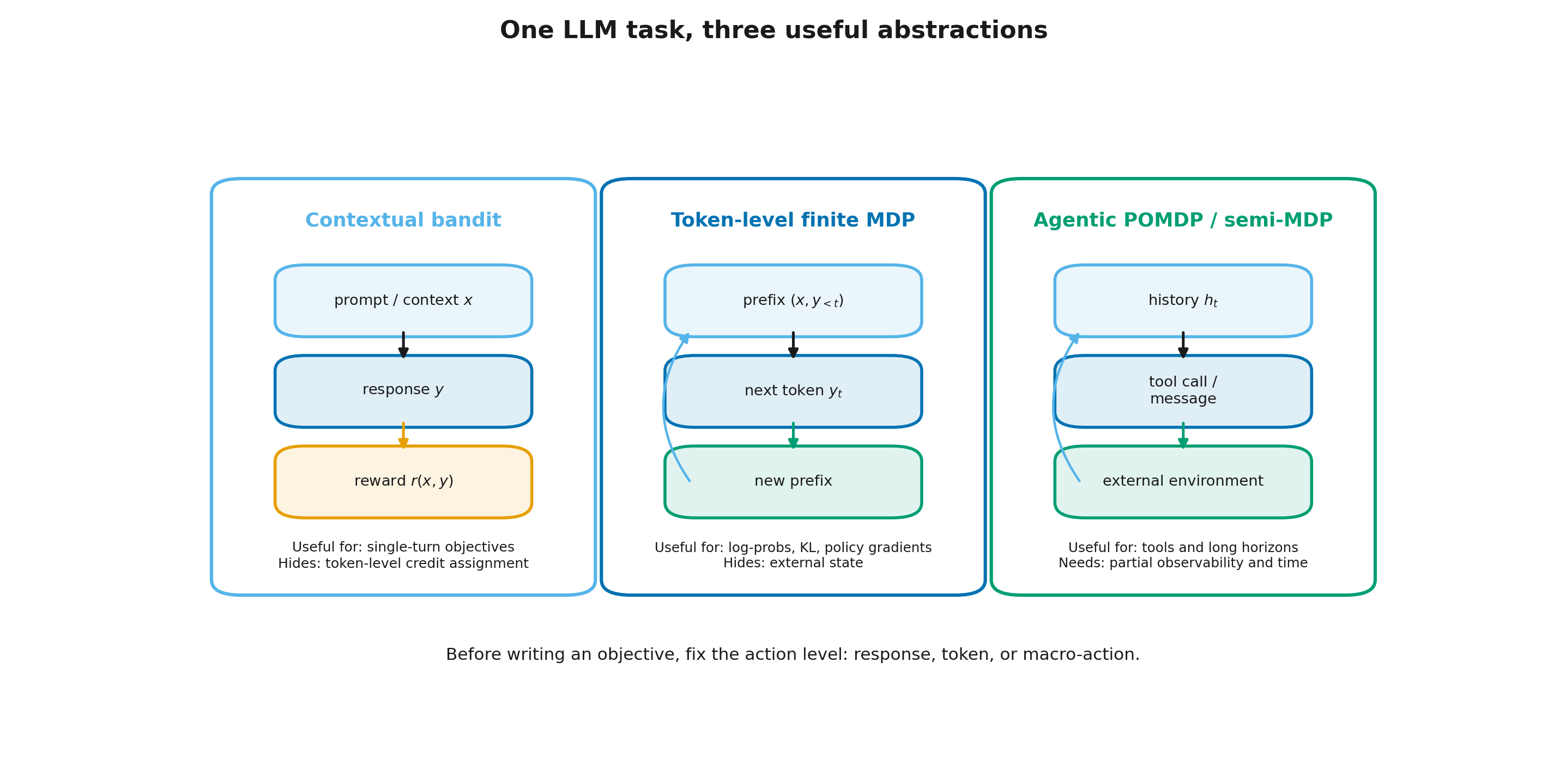
| Formulation | Context or state | Action | Transition | Useful for | What it deliberately hides |
|---|---|---|---|---|---|
| Contextual bandit | prompt | complete response | no next decision is modeled | single-turn preference learning with a terminal reward | token-level credit assignment and decoding cost |
| Finite token-level MDP | full prefix | next token | deterministic token append | log-probabilities, KL, policy gradients, response length | hidden external state and coarse actions |
| Partially observable Markov decision process (POMDP) or semi-Markov decision process (semi-MDP) | observations, history, memory | message, tool call, or macro-action | an external, possibly hidden environment changes | browsers, coding, games, long dialogue | explicit treatment of time, tool failures, and partial observability |
What each name actually claims
The three models differ not in difficulty but in which assumption each one makes and which one it drops.
- MDP assumes the state carries everything relevant to the next transition: how the agent arrived there does not affect what follows. For pure autoregression this holds exactly — the full prefix is the state. The formal definition is given in step 1.1.2.
- POMDP relaxes full observability, not the Markov property of the hidden state. The agent sees not the state but an observation — a partial and possibly noisy projection of it. Part of the world stays hidden: the contents of a file that was never read, the state of a remote service, the user's actual intent. Decisions therefore rest on the interaction history and memory rather than on a single current input.
- semi-MDP drops a different assumption — that every step takes the same amount of time. The "semi-" prefix means the Markov property holds at decision epochs, while arbitrary time may pass between them. An action's duration becomes part of the model alongside its reward: a call taking a second and a call taking a minute stop being the same move.
The token model is an MDP. An agent in a browser or a shell often needs partial observability, and variable action durations may also require a semi-Markov time model. These properties can coexist: accounting for duration does not remove the hidden state.
A complete response as one action
Let be a prompt, a complete response, and a reward. Then
This is a contextual-bandit representation. It is convenient for deriving a response-level objective: one context produces one macro-action and one reward. It does not claim that the response physically appears in one step; internal decoding has been deliberately collapsed.
One token as an action
Let
Until EOS, the transition is deterministic: the selected token is appended to the prefix. This model is natural for log-probabilities, KL, policy gradients, and response length. If the complete prefix contains all information relevant to the selected task, the formulation is Markov.
A message or tool call as an action
After a browser, shell, or test-runner call, the external world changes: a file has been overwritten, a server returned an error, or a user clarified the goal. The transcript need not reveal the entire state, so a POMDP may be more accurate than an MDP. If actions have different durations—for example, one tool call takes a second and another contains a minute of internal work—a semi-MDP may be more natural than a token model.
Course rule: before an important equation, we will state what counts as the state, action, and reward. The same LLM can be a policy in all three formulations, but the meaning of a trajectory and the difficulty of credit assignment change.
Step 1.2.2 — Sparse reward, credit assignment, and rollout cost
A rollout is one trajectory generated by the policy: a complete response or a sequence of agent actions in an environment.
Many LLM tasks reveal the reward only at the end of the rollout:
- did the unit tests pass;
- did the final numerical answer match;
- did the agent complete the browser task;
- did an evaluator prefer one response over another.
Such feedback is a sparse reward, often a terminal reward. If a response contains one thousand tokens and receives only a final or , the credit-assignment problem is immediate: which decisions caused success or failure?
The course will examine several ways to improve the signal.
- A value function and a critic estimate expected future outcomes and provide a more local reference.
- Group baselines compare several responses to the same prompt.
- Process rewards provide intermediate feedback when such feedback can be defined reliably.
- Task decomposition and environment rewards attach feedback to larger actions.
A preview of policy gradients
You can skip this section on a first reading. Module 4 gives the full derivation.
In many policy-gradient methods, the contribution of a selected action has the form
where is the advantage: how much better or worse the selected action was than an expected baseline. In the simplest REINFORCE form, one final return affects the log-probabilities of all actions in the trajectory. The estimator may be unbiased while still having high variance.
None of these methods turns a poor reward into the right objective. Denser or less noisy feedback only helps optimize what was actually specified.
There is also a systems cost. In an abstract token-level MDP, “append a token” is nearly free, but selecting that token requires a forward pass through a large model. For long responses, rollout generation is often the dominant cost. Agentic RL adds tool latency, sandboxing, networking, and retries. Statistical sample efficiency and inference-system throughput therefore meet in one engineering problem.
Lesson 1.3. A Modern Map of LLM Post-Training
Lesson 1.3. A Modern Map of LLM Post-Training
- Where RL sits in the LLM lifecycle
- What changed after classical RL: historical anchors
- Classical axes and their limits
- Five additional coordinates for LLM systems
- Core post-training methods and regimes
- Course route and division of labor with neighboring courses
then 7 assessment steps
Step 1.3.1 — Where RL sits in the LLM lifecycle
A modern LLM is rarely produced by one training regime. We will first expand the names used throughout the rest of the course.
- supervised fine-tuning (SFT), learning from demonstrations;
- reinforcement learning from human feedback (RLHF);
- direct preference optimization (DPO);
- proximal policy optimization (PPO);
- group relative policy optimization (GRPO);
- reinforcement learning with verifiable rewards (RLVR);
- Kullback–Leibler divergence (KL), a measure of distributional difference often used to limit drift from a reference policy.
Five operations should now be kept separate.
| Operation | Data and feedback | Optimized quantity | Fresh generations from the current policy required? | Parameters updated? |
|---|---|---|---|---|
| Pretraining | text sequences; the next token is observed | log-likelihood / cross-entropy | no; the corpus is fixed | yes |
| SFT / behavior cloning | demonstrations of desired responses or actions | demonstration likelihood | no | yes |
| DPO and other direct preference methods | fixed preferred/dispreferred pairs | a pairwise preference loss relative to a reference policy | not during the update itself | yes |
| PPO-RLHF or GRPO/RLVR | responses or trajectories from the current or recent policy plus a reward or verifier | expected reward, often with KL regularization | yes | yes |
| Best-of-N | candidates plus a scorer or verifier | candidate selection with a fixed model | generations are needed for the request | no |
Two conclusions are especially important.
Post-training is not identical to RL. SFT and DPO may be central stages, yet they use fixed data. Best-of-N uses a score but changes no parameters.
An algorithm name does not describe the whole experiment. A complete description should identify who generated the data, which reward was used, how fresh the rollout policy was, how often the batch was reused, and which components were updated.
Further reading: Transformer architecture, pretraining, and SFT are covered in Modern LLMs. They are introduced here only to the depth needed for a self-contained RL route.
Step 1.3.2 — What changed after classical RL: historical anchors
The classical core did not become obsolete. Bellman equations, value functions, policy gradients, exploration, and off-policy correction remain foundational. The application environment changed: actions became tokens and tool calls, rewards became preference models and verifiers, and the cost of collecting experience became the cost of large-model inference.
| Year | Anchor work or line | What carries into this course |
|---|---|---|
| 2015 | deep Q-network (DQN) on Atari | deep value learning and replay as a classical off-policy line |
| 2016–2018 | AlphaGo / AlphaZero | self-play, policy/value learning, and Monte Carlo tree search (MCTS) as distinct system components |
| 2017 | PPO | near/on-policy rollouts and several epochs over a clipped surrogate objective |
| 2022 | InstructGPT | a practical SFT → reward model → PPO-RLHF pipeline |
| 2023 | DPO | a direct pairwise objective from a KL-regularized preference/RLHF formulation |
| 2024 | DeepSeekMath | GRPO: PPO-like optimization with a group baseline and no separately trained critic |
| 2025 | Decoupled Clip and Dynamic sAmpling Policy Optimization (DAPO), GRPO Done Right (Dr. GRPO), and Group Sequence Policy Optimization (GSPO) | different changes to clipping, normalization, group selection, and the level of the importance ratio |
| 2025–2026 | open agentic and model reports | increasing emphasis on interactive environments, tools, and long trajectories |
The primary sources and the precise status of each claim are listed in Module_1_Sources.md.
Frontier snapshot — 2026-07-14. Public reports do not reveal one universal post-training stack. They describe several coexisting families: training on fixed preference data; PPO/GRPO-like optimization on fresh rollouts; RLVR for mathematics and code; and interactive RL for tool use and agentic tasks. Qwen3 reports a unified thinking/non-thinking design; Kimi K2/K2.5 reports joint RL stages including real and synthetic environments; GLM-5 reports asynchronous RL infrastructure and training on long trajectories in agent tasks. These are claims made by primary technical reports, not independent confirmation of a full recipe and not evidence that “the whole industry trains the same way.”
The practical conclusion is narrower: a modern engineer needs classical RL language plus an explicit account of data, feedback, and infrastructure.
Step 1.3.3 — Classical axes and their limits
Classical coordinates remain useful when read as questions.
| Axis | Question | Examples |
|---|---|---|
| model-free / model-based | is a dynamics model used to plan consequences? | PPO is model-free; MCTS with a transition model is model-based planning |
| value-based / policy-based / actor–critic | which object is learned to choose actions? | DQN; REINFORCE; PPO |
| on-policy / off-policy | how closely do the data match the policy being updated? | REINFORCE and PPO are near/on-policy; DQN is off-policy |
| online / offline | are new interactions collected during training? | online RL; offline RL from fixed trajectories |
A short explanation of the second axis:
- Value-based methods learn a state or action value such as , and the policy selects a highly valued action.
- Policy-based methods optimize directly.
- Actor–critic methods learn both an actor policy and a critic/value estimate that helps evaluate actions and reduce variance.
Two pairs are often confused.
On-policy does not mean “use each sample exactly once.” PPO usually collects a batch with and then performs several minibatch epochs while optimizing a surrogate objective with a clipped importance ratio. This clipping does not impose a hard bound on the actual ratio or KL. It is therefore useful to say near/on-policy and report the degree of reuse and policy lag.
Offline is not identical to off-policy. Offline RL is a setting with no further interaction and fixed data. Off-policy is a property of an estimator or algorithm relative to the behavior that produced the data. The concepts are related but answer different questions.
The presence of an LLM does not make a method model-based with respect to the external environment. The system must actually model action consequences and use a transition model for planning.
Step 1.3.4 — Five additional coordinates for LLM systems
The classical map is insufficient for DPO, Best-of-N, and complex agentic pipelines. Ask five additional questions about any system.
- Feedback source: demonstration, preference pair, learned reward, LLM judge, rule-based verifier, or environment outcome?
- Data source: fixed dataset, fresh rollouts from the current policy, rollouts from an older policy, replay buffer, or inference-only candidates?
- Decision unit: token, sequence, tool call, or long trajectory?
- What is updated: policy, critic/value, reward model, reference policy, several components, or nothing?
- Where does optimization occur: in parameters during training or in search and selection during inference?
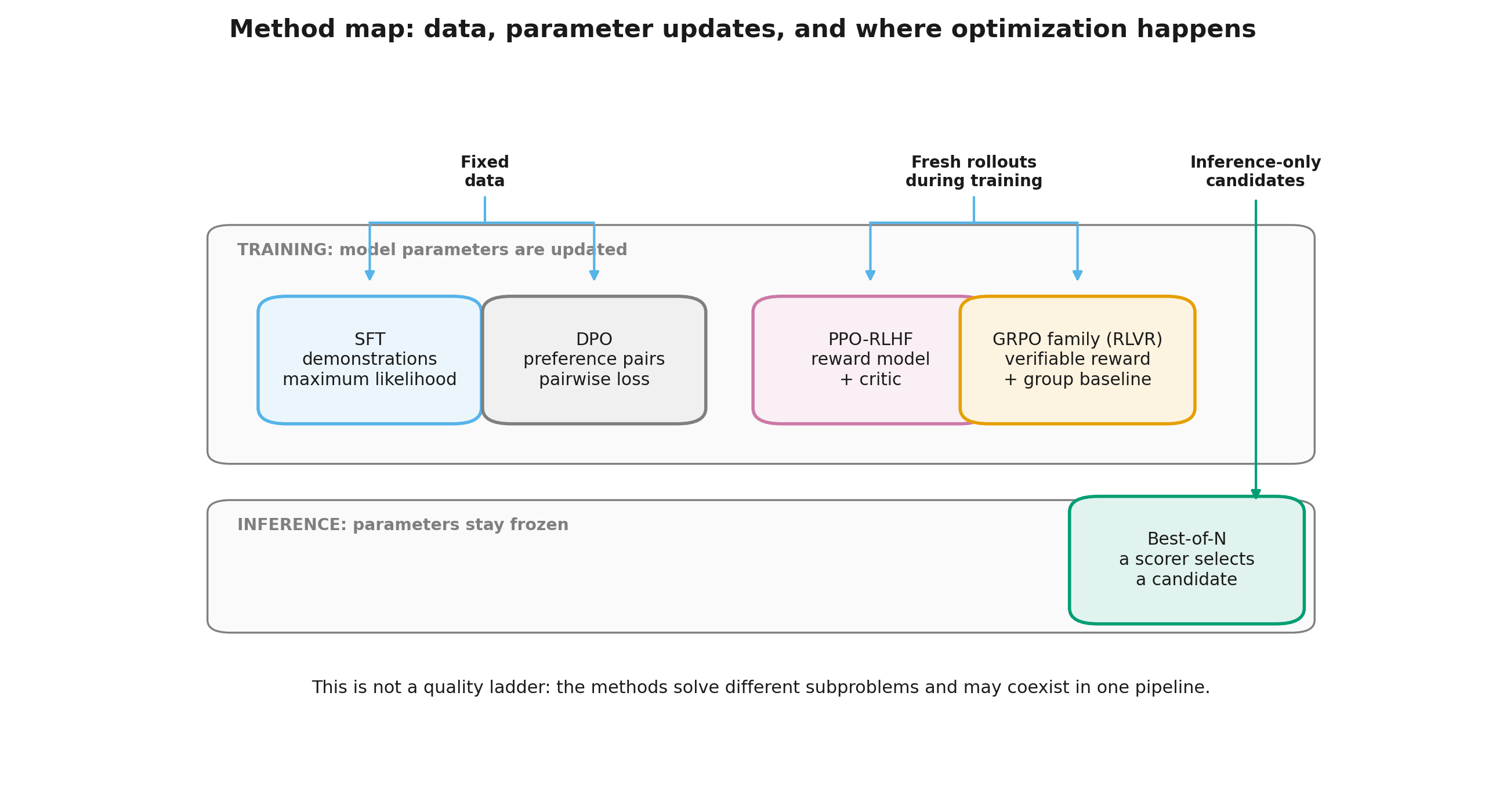
The map is deliberately not a ladder from “worse” to “better.” SFT, DPO, PPO, GRPO, and Best-of-N solve different subproblems and may coexist in one system.
Step 1.3.5 — SFT, DPO, PPO-RLHF, GRPO/RLVR, and Best-of-N
| Method | Data | Feedback and objective | Fresh training rollouts | Additional trainable models | Precise characterization |
|---|---|---|---|---|---|
| SFT | fixed demonstrations | token-level maximum likelihood | no | none | supervised behavior cloning, not RL |
| DPO | fixed preference pairs | a direct pairwise loss relative to a reference policy | no | no separate reward model or critic | offline preference optimization derived from a KL-regularized RLHF formulation; not classical offline RL |
| PPO-RLHF | policy rollouts | learned reward + KL or constraints + PPO surrogate | yes | usually a reward model and critic/value | a near/on-policy actor–critic pipeline |
| GRPO family in RLVR | groups of candidates for one prompt | verifiable or scalar reward + group-relative advantage + PPO-like surrogate | usually yes | canonical GRPO has no learned critic | RLVR describes the feedback regime; GRPO is an algorithm; no critic does not mean no baseline |
| Best-of-N | inference-time candidates | a scorer or verifier selects the best | not a training question | none | inference-time search or selection with frozen parameters |
Why DPO should not simply be called offline RL
DPO uses fixed data and is therefore offline in an ordinary engineering sense. Classical offline RL, however, typically works with transitions or trajectories from a behavior policy, rewards, and Bellman backups; its central problem is improving a policy outside the data distribution. DPO learns from pairwise comparisons and optimizes a different objective. A concise accurate description is direct offline preference optimization derived from a regularized RLHF model.
What on-policy means for PPO and GRPO
Rollouts are usually generated by a snapshot of the current or recent policy , while is updated. The clipped surrogate removes an incentive for certain further ratio changes; it does not guarantee that actual ratios or KL remain within a fixed bound. Multiple epochs and asynchronous rollout systems create some stale or off-policy component; acceptable lag is part of the algorithm specification.
Why there is no single linear branch “after GRPO”
DAPO changes clipping and dynamically removes uninformative groups; Dr. GRPO removes disputed normalizations; GSPO moves the importance ratio and clipping to the sequence level. These are changes to different parts of the estimator and should not be collapsed into “the same GRPO improvement.” Module 9 provides the full derivation and comparison.
Step 1.3.6 — Course route and division of labor with neighboring courses
| Module | Main question |
|---|---|
| 1 | how to enter the RL language and select an LLM formulation |
| 2 | how MDPs, Bellman equations, , and formalize a sequential task |
| 3 | how exploration, bandits, and sampling budgets connect to candidate generation |
| 4 | where policy gradients come from and how REINFORCE leads to PPO |
| 5 | what changes under imitation, off-policy data, and offline RL |
| 6 | how to compute token log-probabilities, KL, and sequence objectives for LLMs |
| 7 | how preference data and reward models are built |
| 8 | how PPO-RLHF, DPO, and direct preference methods work |
| 9 | how GRPO, DAPO, Dr. GRPO, GSPO, and RLVR are derived and stabilized |
| 10 | what belongs to test-time search, process reward models, and inference scaling |
| 11 | how to formulate multi-turn tool and environment interaction |
| 12 | how to separate rollout, inference, and training infrastructure |
| 13 | how to evaluate a policy without self-deception and detect reward hacking |
Cross-references provide depth rather than fill logical gaps.
- Information Theory for ML, Module 2: entropy and units;
- Information Theory for ML, Module 3: cross-entropy and KL;
- Information Theory for ML, Module 8: maximum entropy, softmax, Gibbs tilting, and the exact KL-regularized optimum;
- Modern LLMs: Transformer architecture, pretraining, SFT, inference, and an overview of agents and tool use.
The main RL for LLM text remains self-contained. Stable identifiers are stored in configs/course_links.yaml; public web addresses will be inserted after the repositories are published.
Lesson 1.4. The Practice Contract and First Numerical Experiments
Lesson 1.4. The Practice Contract and First Numerical Experiments
- Four practice tiers
- Temperature softmax: a first computable policy
- Reproducible experiment:
- Return and Monte Carlo evaluation in a corridor
- Takeaways and compact glossary
then 9 assessment steps
Step 1.4.1 — Four practice tiers
Practice does not affect formal course completion. Without running code, however, methods easily remain recognizable words rather than working skills.
We will first expand the computing abbreviations.
- central processing unit (CPU);
- graphics processing unit (GPU);
- application programming interface (API);
- video random-access memory (VRAM), the memory available on a GPU.
| Tier | Environment | Purpose | What counts as a result |
|---|---|---|---|
| A | Quizzes on this site or Stepik; code locally on CPU | functions, mini-MDPs, estimators, unit tests | tests pass and numbers reproduce |
| B | free Colab T4 | smoke or educational run on an open model | notebook runs top to bottom; metrics and configuration are saved |
| B+ | paid API from a major provider | an alternative agent or evaluation route without a large local model | provider, model identifier, date, decoding parameters, raw outputs, and cost are recorded |
| C | paid GPU or multiple GPUs | optional full run or capstone | declared data, steps, checkpoints, and evaluation protocol are completed |
Later DPO, reward-model, GRPO, and agentic-RL exercises will have at least two modes:
- a smoke profile that checks the complete pipeline at small scale;
- a full educational profile that produces a meaningful curve or estimate with honest VRAM, time, and cost reporting.
A smoke run is not presented as a paper reproduction. Module 1 requires only Tier A.
Minimal local setup:
python -m venv .venv
source .venv/bin/activate        # Windows: .venv\Scripts\activate
python -m pip install --upgrade pip
pip install numpy matplotlib
Checked reference code is in module_1_reference.py.
Step 1.4.2 — Temperature softmax: a first computable policy
Suppose the model produces logits . A logit is an unnormalized action score. The temperature policy is
A numerically stable form subtracts the largest logit:
Small concentrates probability on high-logit actions. Large makes the distribution more uniform. This is one of the simplest ways to see a policy as a complete distribution rather than as “the selected token.”
The policy entropy in nats is
For fixed finite logits with no top-k, top-p, or other transformations, entropy is nondecreasing in temperature:
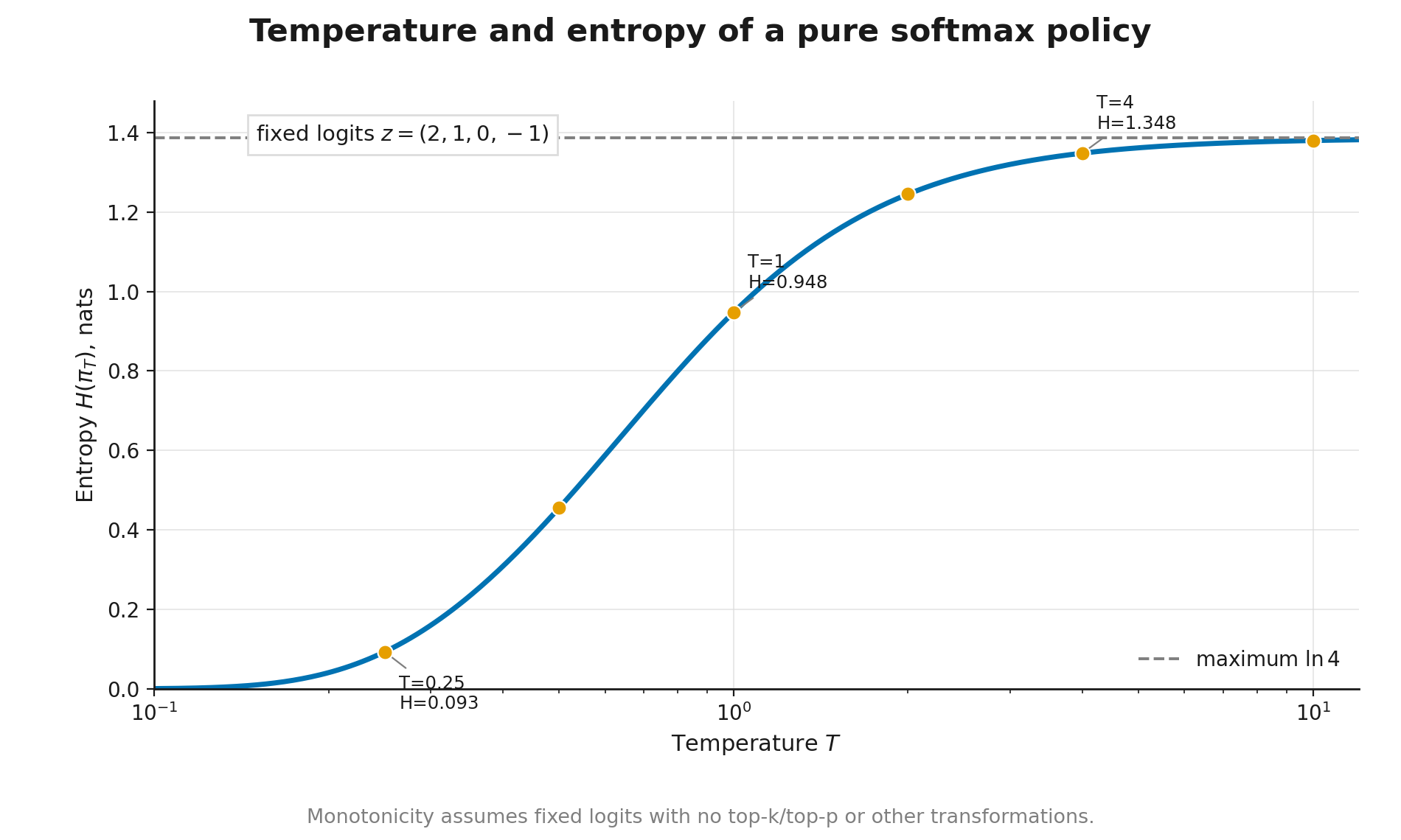
Boundary of the statement. A real API may combine temperature with top-p, top-k, repetition penalties, safety filters, and provider-specific transformations. The equation describes pure temperature softmax applied to a given set of logits, not the entire decoding pipeline.
Further reading: Information Theory for ML, Module 2 covers entropy; Module 8 derives softmax as a maximum-entropy or Gibbs solution.
Step 1.4.3 — Reproducible experiment:
For logits :
| , nats | ||
|---|---|---|
| 0.25 | 0.093113 | 0.0672 |
| 0.50 | 0.455429 | 0.3285 |
| 1.00 | 0.947537 | 0.6835 |
| 2.00 | 1.245050 | 0.8981 |
| 4.00 | 1.348243 | 0.9726 |
| 10.00 | 1.380071 | 0.9955 |
Minimal code:
from __future__ import annotations

import numpy as np

def softmax_with_temperature(logits: np.ndarray, temperature: float) -> np.ndarray:
    logits = np.asarray(logits, dtype=np.float64)
    if logits.ndim != 1 or logits.size == 0:
        raise ValueError("logits must be a non-empty 1D array")
    if not np.isfinite(logits).all():
        raise ValueError("logits must be finite")
    if not np.isfinite(temperature) or temperature <= 0:
        raise ValueError("temperature must be finite and positive")

    scaled = logits / temperature
    scaled -= scaled.max()
    weights = np.exp(scaled)
    return weights / weights.sum()

def policy_entropy(logits: np.ndarray, temperature: float) -> float:
    p = softmax_with_temperature(logits, temperature)
    positive = p > 0
    return float(-(p[positive] * np.log(p[positive])).sum())
In the practice material, these functions become small checked exercises with worked explanations. They test not only the formula but numerical hygiene: , an empty vector, and nan must raise clear errors, while logits around 1000 must still produce finite probabilities.
Step 1.4.4 — Return and Monte Carlo evaluation in a corridor
The classical example is a symmetric random walk over five cells:
terminal           start             terminal, reward +1
   [0] ---- [1] ---- [2] ---- [3] ---- [4]
Action 0 moves left and action 1 moves right. The episode ends at 0 or 4; reaching 4 gives reward .
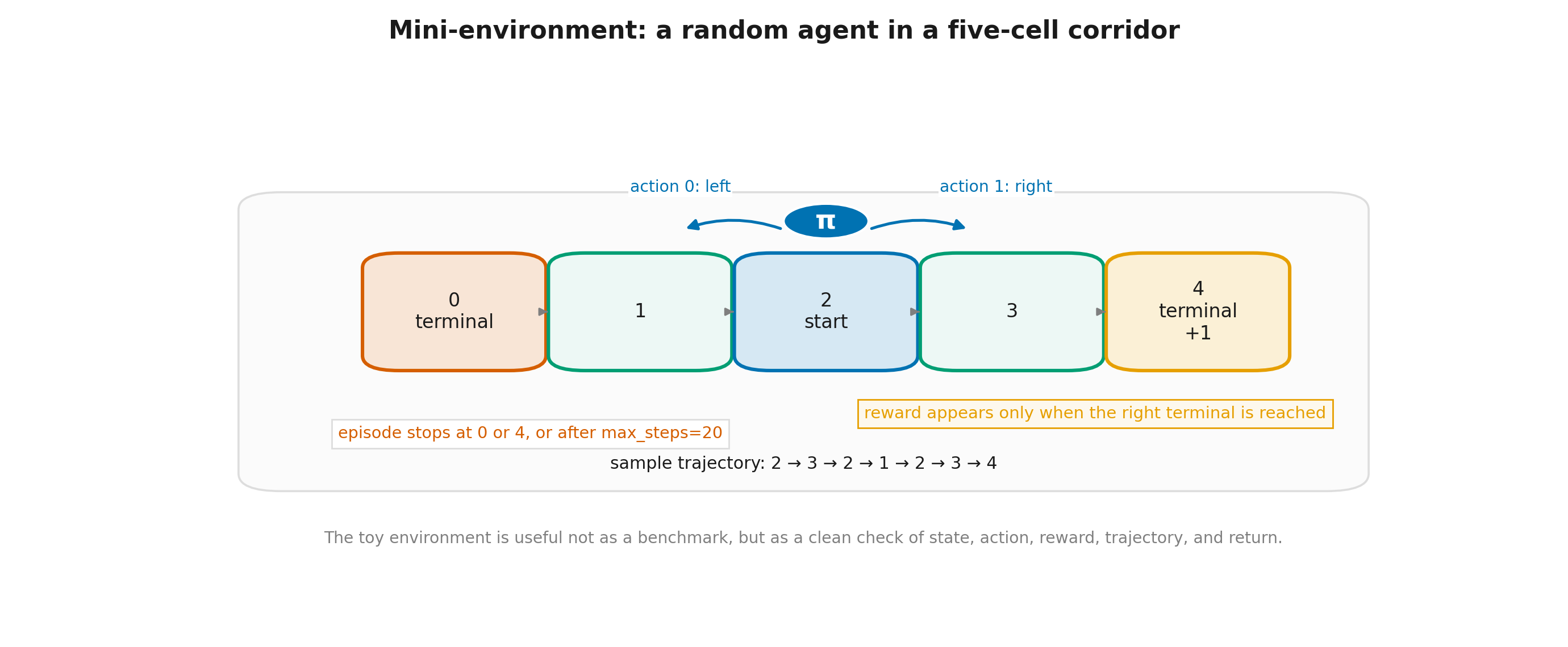
The corridor is intentionally small, but it already contains the RL objects we need: the state is the current cell, the action is a left-or-right step, the reward is the event of reaching the right terminal, and a trajectory is the whole path before stopping. The point is not that this is a realistic environment; the point is that the formula can be checked before we transfer the same logic to tokens, responses, and LLM rollouts.
The state-value function is expected return from a state:
Without an artificial length limit, an equiprobable random policy starting in the center has
The code truncates an episode after 20 actions, so the exact value of the executed protocol is slightly smaller:
The difference is small but methodologically important: compare an experiment with the task that was actually run, not with a nearly identical infinite-horizon version.
The Monte Carlo method estimates an expectation by an average over independent episodes:
Here the return is Bernoulli with , so the standard error at is approximately
Values such as 0.48, 0.50, and 0.52 do not contradict the theory; they reflect finite-sample noise. With , seed=7, and max_steps=20, the reference code returns 0.494.
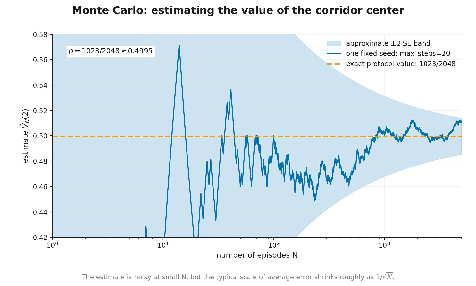
The plot should not be read as a promise of neat monotone convergence: a finite estimate can sit above or below the exact value. The useful lesson is that the noise of an average over independent episodes shrinks on the order of , while the horizon and stopping rule must match the protocol actually implemented in code.
The same logic will return in verifiable-reward training: several rollouts for one prompt provide a random quality estimate, and group size affects both variance and cost.
Step 1.4.5 — Takeaways and compact glossary
Module 1 leaves us with a minimal but already precise map.
- An agent acts in an environment, receives rewards, and produces trajectories.
- A policy is a distribution over actions; under a token-level abstraction, an LLM exactly defines .
- A reward belongs to a transition; a return is an accumulated future outcome.
- In online RL, the policy changes the distribution of the next experience.
- A complete response can be modeled as a contextual bandit, token generation as an MDP, and a tool-using agent as a POMDP or semi-MDP.
- SFT, DPO, PPO-RLHF, GRPO/RLVR, and Best-of-N differ in data, feedback, updated components, and optimization location.
- The temperature result concerns pure softmax; a real decoding pipeline is broader.
- A more convenient reward or a larger rollout budget does not prove that the objective itself is correct.
Compact acronym glossary:
| Acronym | Full name | Role in the course |
|---|---|---|
| RL | reinforcement learning | policy learning from feedback and return |
| LLM | large language model | a model that can parameterize a policy |
| MDP | Markov decision process | a fully observed sequential model |
| POMDP | partially observable Markov decision process | a model with hidden state and observations |
| semi-MDP | semi-Markov decision process | a model in which actions have different durations |
| SFT | supervised fine-tuning | behavior cloning from demonstrations |
| RLHF | reinforcement learning from human feedback | an RL pipeline using human preferences |
| DPO | direct preference optimization | direct pairwise optimization from fixed preferences |
| PPO | proximal policy optimization | a near/on-policy policy-optimization algorithm |
| GRPO | group relative policy optimization | a PPO-like method with a group baseline and no learned critic |
| RLVR | reinforcement learning with verifiable rewards | RL with automatically checkable rewards |
| KL | Kullback–Leibler divergence | a measure of policy deviation from a reference |
| API | application programming interface | an external software interface to a model or tool |
Exit check: answer the conceptual questions and complete four Tier-A exercises: return, stable softmax, entropy, and Monte Carlo evaluation. On the learning platform, every item is followed by a worked explanation after the learner has attempted it. Practice is optional for formal completion, but it is what turns definitions into working habits.
Next — Module 2: MDPs, Bellman equations, and functions, prediction, and tabular control. It formalizes the sequential part of the map introduced here in words.
Sources and Currency Status
The list below is a short reading route for the claims made in this module. The complete bilingual registry — including claim status, verification date, and explicit limitations — is in Module_1_Sources.md.
- Richard S. Sutton and Andrew G. Barto. Reinforcement Learning: An Introduction, 2nd ed. — the foundational source for MDPs, policies, returns, value functions, and Monte Carlo evaluation. It is an RL textbook, not a recipe for LLM post-training.
- John Schulman et al. Proximal Policy Optimization Algorithms — the primary PPO paper: rollout collection, several minibatch epochs over one batch, and the clipped surrogate objective. The module’s “near/on-policy” wording should be read together with batch reuse and possible policy lag.
- Long Ouyang et al. Training language models to follow instructions with human feedback — the authors’ account of the InstructGPT SFT → ranking-based reward model → PPO-RLHF pipeline. It is a historically important implementation, not a universal mandatory sequence.
- Rafael Rafailov et al. Direct Preference Optimization: Your Language Model is Secretly a Reward Model — the source for DPO, its pairwise objective, and its connection to a KL-regularized preference formulation. The course deliberately does not relabel DPO as classical offline RL.
- Zhihong Shao et al. DeepSeekMath: Pushing the Limits of Mathematical Reasoning in Open Language Models — introduces GRPO as a PPO-like method with group-relative estimates and no separately trained critic. No critic does not mean no baseline.
- DeepSeek-AI. DeepSeek-R1: Incentivizing Reasoning Capability in LLMs via Reinforcement Learning — an author-reported large-scale RL/GRPO recipe for reasoning, with a distinction between R1-Zero and the multi-stage R1 system. Its results and interpretations are not a complete independent replication.
- Zichen Liu et al. Understanding R1-Zero-Like Training: A Critical Perspective — a useful qualification of the GRPO family, analyzing consequences of selected normalizations and proposing Dr. GRPO. Its conclusions concern a particular estimator and objective, not a universal guarantee of “unbiased RL.”
The contemporary examples in the lecture form a dated snapshot, not a model leaderboard and not a claim that one post-training architecture has become universally correct. For those entries, the “Boundary / limitation” column in the full registry is part of the citation.