Module 12. RL infrastructure for LLMs: memory, rollouts, and asynchrony
Material version: 2026.24
Factual snapshot: 2026-08-06
Language: EN
Core practice: profile A — browser and central processing unit (CPU); profile B — a free Colab T4; profile C — an optional multi-GPU run
Structure: 5 lessons, 25 steps
Estimated time: 10–12 hours without the optional model run
Modules 8–11 developed objectives, group rollouts, verifiable rewards, and long agent trajectories. The last topic is treated directly in RL for LLM, Module 11 “RL for LLM Agents: Tools, Environments, and Long Trajectories” (rl_llm.module_11_agentic_rl). The engineering question is now unavoidable: how do we turn these formulas into a system that collects data, updates a model, and preserves the meaning of the behavior policy while information moves between programs?
Follow one rollout through the machine. It begins as a scheduler record, becomes an inference request, accumulates tokens and KV-cache state, passes through a verifier, waits in a queue, enters a training batch, contributes to a gradient, and must finally be attributable to a published weight version. Losing a mask, policy version, actual behavior log-probability, or reward provenance at any boundary changes the statistical object, not merely the software quality.
The same GRPO objective can run as a sequential one-GPU script, a pipeline with separate rollout and training pools, or a fully asynchronous queue. The algorithmic mechanics are developed in RL for LLM, Module 9 “RLVR and GRPO: Verifiable Rewards, Group-Relative Estimates, and Stability” (rl_llm.module_09_rlvr_grpo). This module studies the systems layer: different executions create different memory peaks, lag distributions, and risks of stale or incorrectly attributed data.
The practical task of this module is:
Design and measure an RL loop in which generation, training, weight synchronization, rollout logging, and failure recovery form one auditable system with controlled memory, throughput, and staleness.
By the end of the module, you will be able to:
- represent an RL loop as a dataflow among a policy, rollout engine, verifier, trainer, and storage;
- distinguish colocated from disaggregated placement;
- separate algorithmic synchrony from physical process placement;
- define a minimal rollout contract with a behavior-policy version;
- account for parameters, gradients, and Adam state without assuming one universal byte count per parameter;
- explain what Fully Sharded Data Parallel (FSDP) and Zero Redundancy Optimizer (ZeRO) shard and which peaks remain;
- estimate key–value cache (KV-cache) memory from architecture and retained tokens;
- distinguish training memory, generation memory, and the time-dependent peak of colocation;
- compute sequential and overlapped pipeline time;
- measure loss of utilization from variable completion length and stragglers;
- state a first-order queue-stability condition and introduce backpressure;
- distinguish policy lag from training–inference mismatch;
- compute probability ratios, clipping statistics, and effective sample size (ESS);
- choose among log-probability recomputation, importance correction, and stale-data rejection;
- design atomic synchronization for full weights or adapters;
- define a complete RL-run checkpoint and test recovery before failure;
- trace a prompt through rollout, weight version, reward, batch, and optimizer step;
- compare TRL, verl, OpenRLHF, NeMo RL, PRIME-RL, SkyRL, and AReaL along architectural axes rather than one ranking;
- profile a synthetic RL pipeline on CPU and optionally a small open model on a Colab T4.
Practice route. Graded tasks, worked solutions revealed after an attempt, and executable practice follow the lecture. The explanation remains self-contained.
Lesson 12.1. The RL loop as a dataflow
Lesson 12.1. The RL loop as a dataflow
- Why one
trainer.generate()call is not enough- The role contract matters more than the queue format
- Placement and synchrony are independent axes
- The behavior policy needs an atomic rollout version
- Measure a sequential baseline before building a distributed system
then 2 assessment steps
Step 12.1.1 — Why one trainer.generate() call is not enough
Start with the physical loop rather than a framework name. One online-RL update needs to:
- select a prompt or environment state;
- obtain one or more rollouts from the behavior policy;
- compute rewards and operational status;
- recover masks and log-probabilities;
- assemble a training batch;
- compute the loss and gradients;
- update parameters;
- make the new policy version available to data collectors.
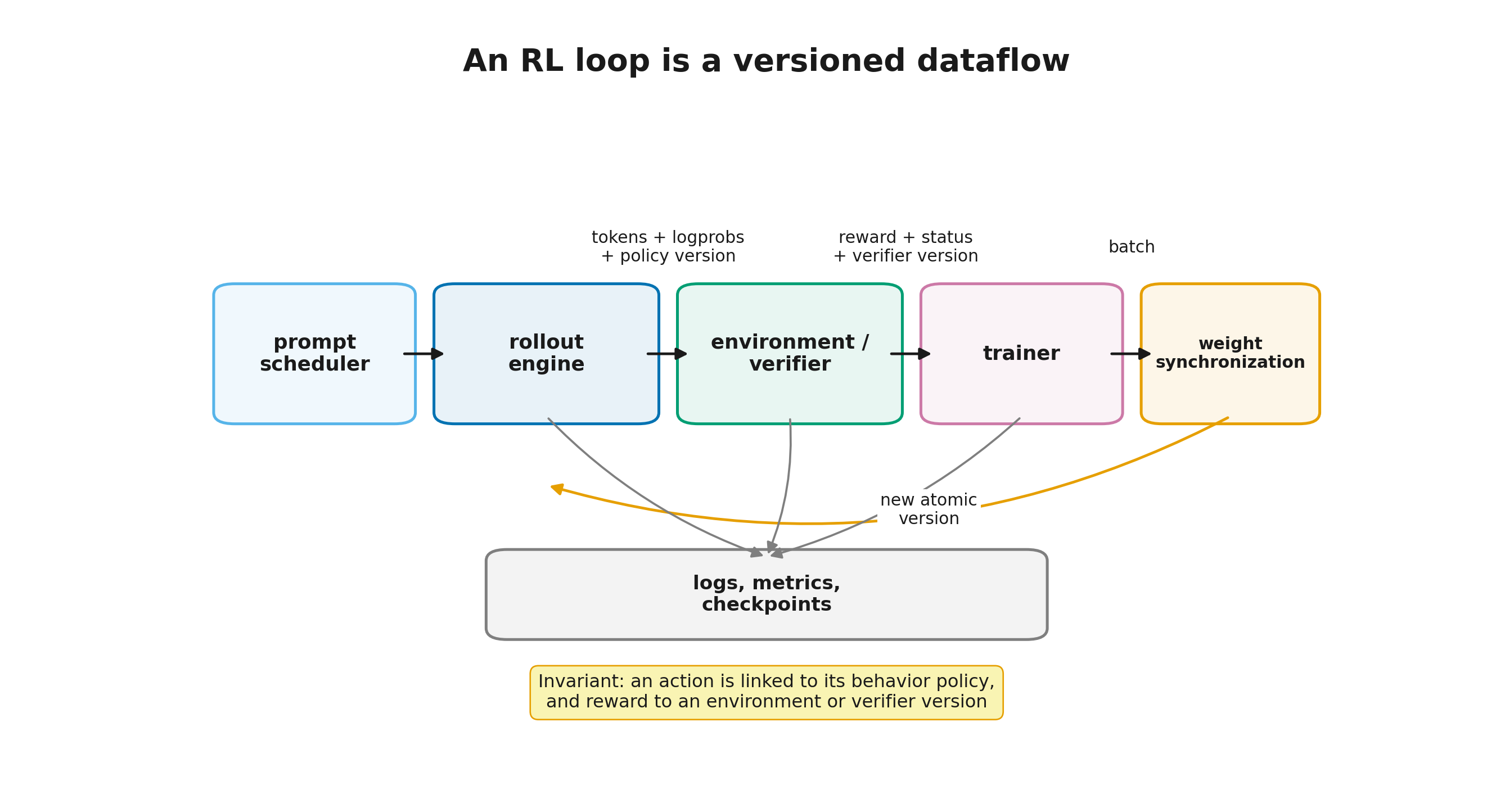
A small script can perform every role in one process. At scale, the roles become separate programs or worker groups:
- a prompt scheduler selects tasks;
- a rollout engine decodes efficiently;
- an environment or verifier computes outcomes;
- a trainer runs forward and backward passes;
- a synchronization service publishes a new weight version;
- storage and telemetry preserve experience, metrics, and checkpoints.
This decomposition is not a theorem. It appears because generation and training have different computational profiles.
- Decode performs many short sequential steps, while KV-cache memory follows the number and length of active sequences.
- Training benefits from dense batches, saved activations, backward computation, and gradient collectives.
An inference engine such as vLLM or SGLang and a trainer built on FSDP, DeepSpeed, or Megatron may serve the same policy while solving different systems problems.
Boundary. A training library can generate text, and an inference engine can execute a forward pass. Role separation is an engineering choice, not an impossibility result. A sequential one-GPU script is often the best control because it has fewer moving parts.
Step 12.1.2 — The role contract matters more than the queue format
Passing only an answer string between two processes is insufficient for a correct policy update. A minimal rollout record must answer at least the following questions.
| Field | Why it is needed |
|---|---|
sample_id, prompt_id | connect a prompt, its answer group, and later diagnosis |
| token IDs | reconstruct the exact policy actions |
| policy-token mask | avoid training on environment or template text |
| behavior log-probabilities | compute probability ratios or test stack agreement |
policy_version | measure policy lag |
| decoding parameters | reconstruct the actual behavior distribution |
| reward components | separate task outcome from format and cost terms |
| stop reason | distinguish the end-of-sequence token (EOS), limits, task failure, and infrastructure failure |
| verifier version | avoid silently mixing reward specifications |
| timestamps | measure queueing, rollout, verification, and training |
A record may look like this:
{
  "sample_id": "run42-p008-g03",
  "policy_version": 127,
  "prompt_tokens": [101, 42, 17],
  "response_tokens": [314, 159, 2],
  "policy_mask": [0, 0, 0, 1, 1, 1],
  "behavior_logprobs": [-0.31, -1.07, -0.22],
  "decoding": {"temperature": 0.8, "top_p": 1.0},
  "reward": {"correctness": 1.0, "format": 0.0},
  "stop_reason": "eos",
  "verifier_version": "arith-v4"
}
The physical container need not be JSON. Apache Arrow, Parquet, a message queue, or an in-memory object can all work. What matters is preserved semantics.
Module 11 introduced token provenance in a multi-turn trajectory. The systems requirement is stronger: provenance must survive serialization, queuing, and process restart. If a record cannot distinguish policy tokens from environment observations after reload, no trainer can recover an honest loss.
Step 12.1.3 — Placement and synchrony are independent axes
Infrastructure is easier to reason about when two commonly conflated axes are separated.
Axis 1 — computational placement.
- Colocation: rollout and training alternate on the same graphics processing units (GPUs). It lowers the minimum device count and can simplify weight publication, but the roles compete for memory and cannot use the same device simultaneously.
- Disaggregation: rollout engines and trainers occupy different GPUs or nodes. Work can overlap and pools can scale independently, but the design adds networking, weight transfer, queues, and staleness.
Axis 2 — data and update order.
- Synchronous mode: the trainer waits for a defined rollout batch, updates, and then starts the next logical cycle.
- Asynchronous mode: collectors keep producing while the trainer updates; records arrive from multiple policy versions.
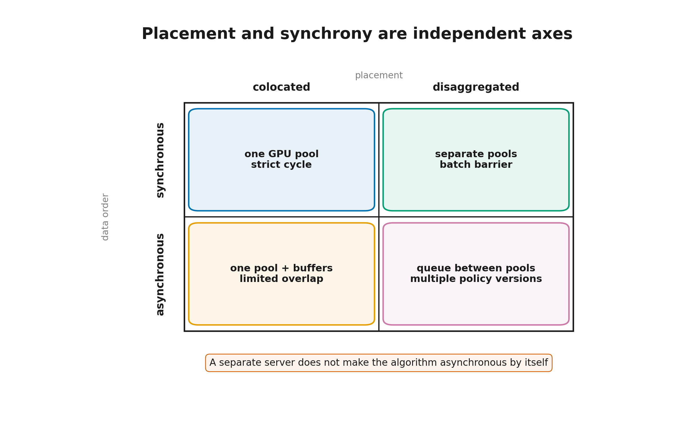
The axes are independent.
- Colocation is usually sequential, but CPU-side preparation and buffering may overlap.
- Disaggregated pools may remain strictly synchronous: the rollout pool creates a batch and then waits for training and synchronization.
- Disaggregated pools may be fully asynchronous with an age-bounded queue.
This map prevents the false conclusion that “a separate vLLM server automatically makes the algorithm asynchronous.” A physically separate server can still participate in a strict barrier protocol.
For a first reproducible experiment, begin in the simplest cell: one process, one batch, one policy version. Every later complication should be justified by a measured bottleneck.
Step 12.1.4 — The behavior policy needs an atomic rollout version
Suppose the rollout engine uses weight version , while the trainer has already reached version . Write the actual behavior policy as
and the current trainable policy as
In a synchronous run, when data collection begins, although Proximal Policy Optimization (PPO) may update the current policy relative to a frozen old policy over several epochs. In an asynchronous run, the difference
is the policy lag.
A version should refer to a concrete probability distribution, not merely a filename. Three safe regimes are possible.
- One version per completion. In-flight requests finish under the old weights, and the engine atomically switches before accepting new requests.
- One version per agent turn. This can be valid for long episodes if the log stores the version and behavior log-probabilities of every action.
- The exact behavior policy is recorded. If weights change in the middle of a completion, token-level versions and probabilities plus an unambiguous update order are required; analysis becomes substantially harder.
The first regime is usually simplest for one-shot completions. Long multi-turn agents may require the second.
Invariant: a rollout cannot be labeled with one version if its actions were actually sampled from several versions.
Atomicity also includes decoding. Temperature, top-p, forbidden tokens, and EOS handling are part of the behavior policy. Identical weights with different decoding rules define different distributions.
Step 12.1.5 — Measure a sequential baseline before building a distributed system
Before choosing Ray, Kubernetes, or a multi-process engine, measure one sequential control loop. For every batch, log:
- prompt preparation time;
- prefill time;
- decode time;
- verifier time;
- log-probability recomputation;
- forward and backward time;
- optimizer-step time;
- weight-synchronization time;
- input and output token counts;
- peak memory.
The sequential cycle is
This is accounting, not a cluster-performance model. It answers the first question: which stage actually dominates this configuration?
“Generation is always the bottleneck” is too strong. It is often true for long reasoning traces and few training epochs, but can fail with short outputs, many epochs, a heavy critic, slow verification, or expensive weight transfer.
The optional notebook first constructs this synthetic profile. Its real-model branch then measures generation and a teacher-forced forward pass on a small open model. That branch teaches timers and units; it is not a benchmark of a large cluster.
Lesson 12.2. Memory and throughput
Lesson 12.2. Memory and throughput
- “Sixteen bytes per parameter” is a profile, not a law
- Replication, FSDP, and ZeRO
- Engine memory: weights and KV cache
- Colocation requires a time-dependent memory ledger
- Throughput needs tokens and events, not one example count
then 3 assessment steps
Step 12.2.1 — “Sixteen bytes per parameter” is a profile, not a law
A common estimate says mixed-precision Adam training needs about 16 bytes per parameter. It is useful as one scenario and dangerous as a universal constant.
Logical model-state memory is the sum of representations that are actually stored:
where is parameter count and each is bytes per parameter of the corresponding object.
One common profile is:
| Component | Type | Bytes/parameter |
|---|---|---|
| working parameters | bfloat16 | 2 |
| gradients | bfloat16 | 2 |
| first Adam moment | float32 | 4 |
| second Adam moment | float32 | 4 |
| separate master copy | float32 | 0 or 4 |
| Total | 12 or 16 |
The range exists because implementations differ.
- Some keep a separate float32 master copy; others treat another high-precision shard as the canonical state.
- Gradients may be bfloat16 or float32.
- Optimizer states may be quantized, offloaded, or replaced by another optimizer.
- Adapter training stores optimizer state only for a small trainable subset.
Model state is not the whole device footprint. Activations, collective buffers, logits, masks, KV cache, allocator fragmentation, and environment memory remain. Bytes per parameter are the first line of a budget, not the answer to “will this run fit?”
Step 12.2.2 — Replication, FSDP, and ZeRO
With Distributed Data Parallel (DDP), every process holds a full model and optimizer-state replica. Each process receives different examples and gradients are reduced across replicas.
Fully Sharded Data Parallel (FSDP) and the Zero Redundancy Optimizer (ZeRO) reduce model-state replication. In their most complete forms, parameters, gradients, and optimizer state are partitioned across data-parallel participants.
A first-order persistent footprint is
The approximation sign is essential. During forward and backward passes, modules may be gathered temporarily, communication buffers are allocated, and large objects may not align perfectly with the shard boundary. Peak memory depends on:
- wrapping and shard boundaries;
- the largest materialized module;
- prefetching;
- activation checkpointing;
- concurrent microbatches;
- logit computation;
- the communication backend.
Therefore is an order-of-magnitude check, not a substitute for a memory trace.
Extension: general DDP, FSDP/ZeRO, tensor parallelism, and pipeline parallelism are developed in Modern LLMs, Module 9 “Pretraining: Data, Scaling Laws, and Optimizers” (
modern_llms.module_08_pretraining). The additional concern here is the rollout engine and movement of one policy between training and generation layouts.
Step 12.2.3 — Engine memory: weights and KV cache
A rollout engine normally stores no gradients or optimizer states. Its largest components are:
- model weights;
- the KV cache of active sequences;
- temporary workspaces and graphs;
- sometimes several adapter or weight versions.
For a transformer with layers, key–value heads, head dimension , and retained tokens,
where the factor two accounts for keys and values and is bytes per element.
Consider
One retained token needs
Sixty-four sequences of 4096 tokens contain 262144 retained tokens and require exactly 32 GiB of useful KV payload in this simplified architecture.
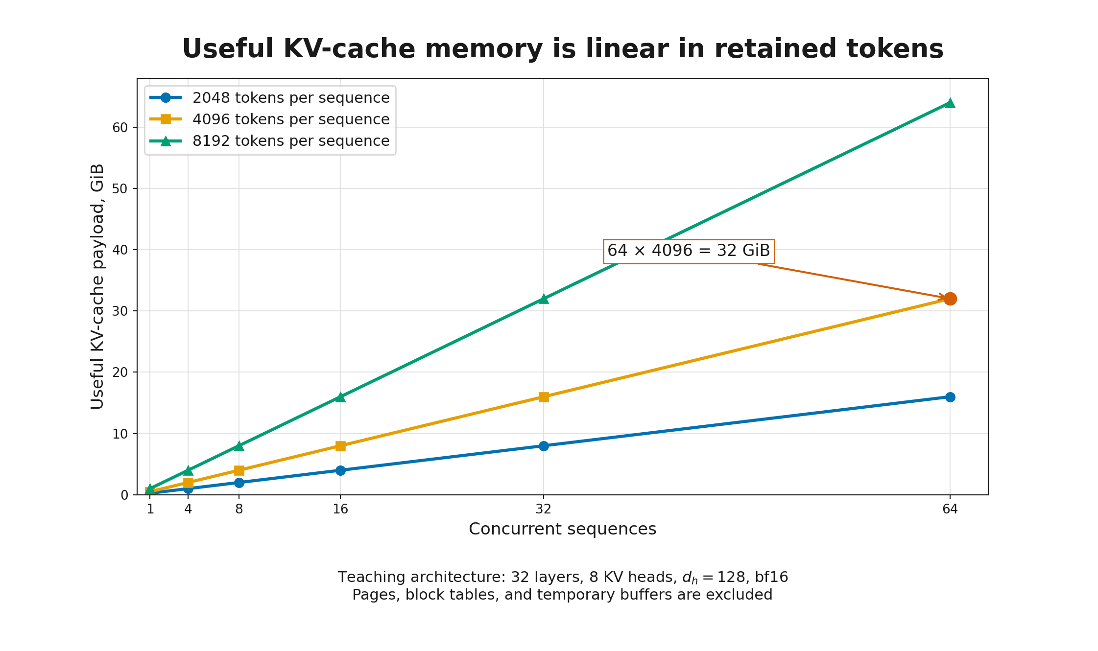
This explains why GRPO group size and reasoning length are infrastructure parameters: more candidates increase active sequence count, and long completions hold pages longer.
PagedAttention reduces fragmentation in vLLM; RadixAttention in SGLang can reuse common prefixes. Neither removes the linear payload of retained keys and values.
Extension: multi-query, grouped-query, and multi-head latent attention, PagedAttention, prefix caching, and distributed serving are developed in Modern LLMs, Module 10 “KV Caches and Efficient Inference” (
modern_llms.module_09_inference).
Step 12.2.4 — Colocation requires a time-dependent memory ledger
With disaggregation, trainer and rollout engine occupy different GPUs. Their memory contributes to cluster total but not to one device peak.
With colocation, the same GPU pool alternates roles. Simply adding both phase maxima is too pessimistic because some objects can sleep, offload, or be freed between phases. The correct object is a timeline.
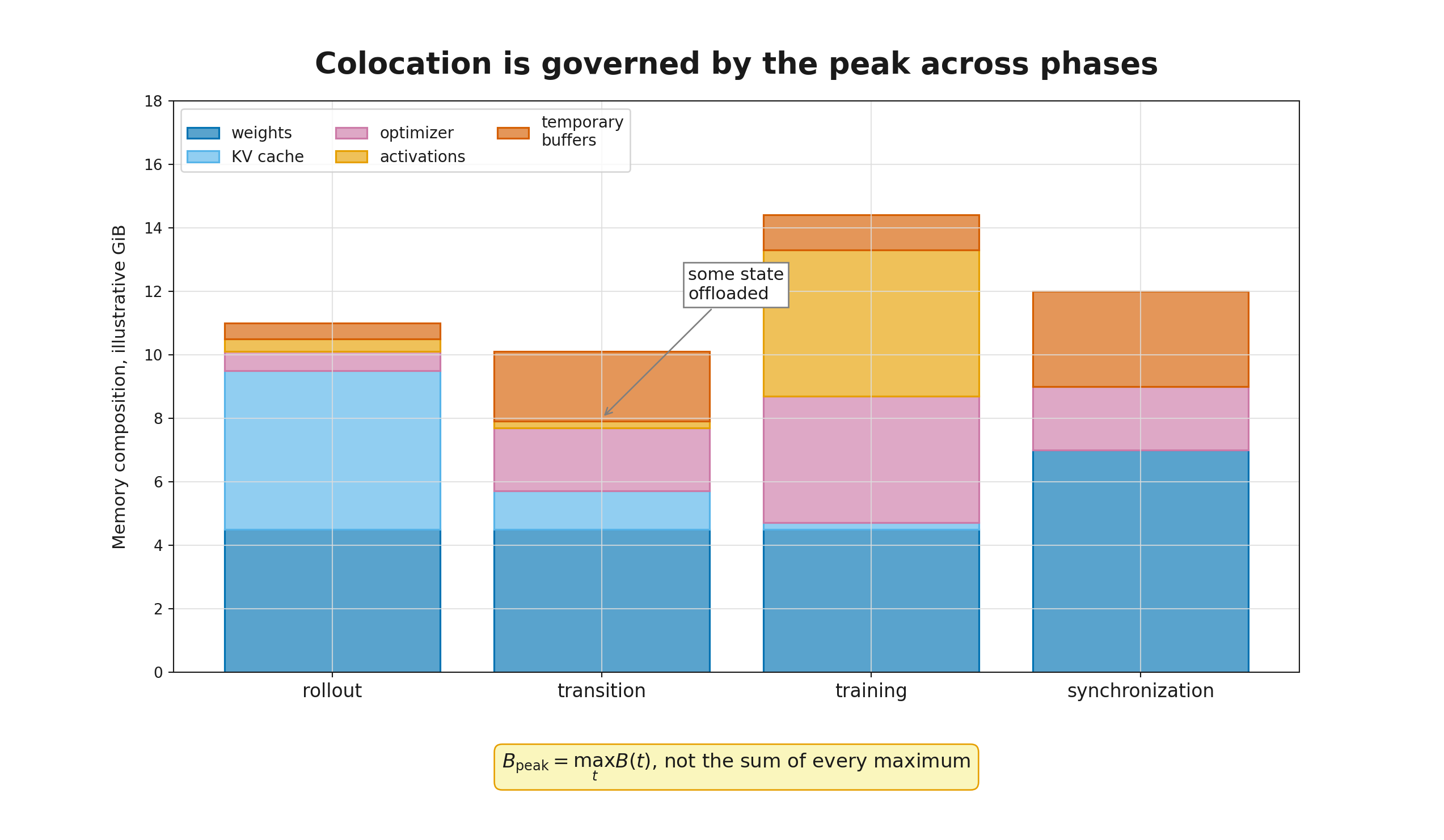
A typical sequence is:
- Rollout: engine-format weights and a large KV cache are active; optimizer state may be sharded, offloaded, or put to sleep.
- Transition: the KV cache is released or reduced and trainer state becomes active.
- Training: parameters, gradients, optimizer state, and activations are active; most engine workspace is released.
- Synchronization: the new weight version is transformed or loaded into the engine representation.
The peak is
including transition buffers.
LoRA changes two parts of the ledger.
- Gradients and optimizer states exist only for adapters.
- Base weights still support every forward pass, and the rollout engine must receive a consistent adapter version or merged representation.
LoRA can make colocation practical, but it does not make rollout memory vanish. The exact adapter-update path remains a versioned library feature.
Step 12.2.5 — Throughput needs tokens and events, not one example count
“Examples per second” is a poor comparison when prompts and completions differ in length. A minimal report separates:
- input tokens per second;
- output tokens per second;
- completed rollouts per second;
- verified outcomes per second;
- training tokens per second;
- optimizer steps per hour;
- cost per informative update.
For rollout, prefill and inter-token decode time should be separated. For training, count non-padding policy tokens, not only packed sequence length.
A generic throughput is
But useful work depends on the question. If 90% of groups have equal reward, high output-token throughput does not imply high learning-signal throughput. A systems dashboard can therefore include
This is not a task-quality metric. It explains why expensive hardware may produce many tokens but few non-zero relative advantages.
Lesson 12.3. Pipelines, queues, and stragglers
Lesson 12.3. Pipelines, queues, and stragglers
- Sequential loop and overlapped pipeline
- Mean time hides slow tails
- Continuous batching and prefix reuse
- Queue stability and backpressure
- Profile the timeline before interpreting GPU utilization
then 4 assessment steps
Step 12.3.1 — Sequential loop and overlapped pipeline
Let one logical batch have two large stages:
- rollout plus reward takes seconds;
- training plus synchronization takes seconds.
Sequential cycle time is
If the stages occupy independent resources and overlap, the steady-state period after filling the two-stage pipeline is
For batches, ideal total time is
The first batch still traverses both stages; throughput improves only over a stream.
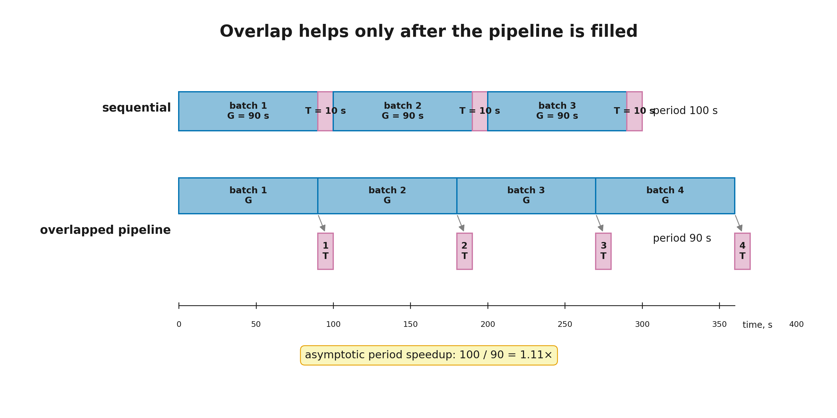
Two-stage speedup approaches two only when . If rollout takes 90 seconds and training takes 10, the period falls from 100 to 90 seconds, only . The fast trainer spends most of its time waiting for data.
Pool sizes should therefore follow measured stage rates rather than an equal split of GPUs. Add resources to the stage that limits the period until another bottleneck—network, verifier, or memory—appears.
Step 12.3.2 — Mean time hides slow tails
A group method often waits for completions of one prompt. With parallel rollout, group time is the maximum:
Suppose eight rollouts take
Total work is 55 GPU-seconds, but eight workers are reserved for 20 seconds. Utilization relative to the ideal rectangle is
One long completion leaves most resources idle.
Long tails come from completion length, tool calls, environment timeouts, prompt size, retries, and uneven routing. Remedies include cost-aware bucketing, continuous batching, explicit turn/time budgets, streaming completed rollouts, and separating infrastructure retries from policy actions.
Truncating the tail saves wall time but changes data. If hard tasks are systematically longer, unconditional removal biases training toward easy cases. Timeout rules and truncation rates belong in the experiment report.
Step 12.3.3 — Continuous batching and prefix reuse
An inference engine is valuable not merely because it “can generate,” but because it schedules many requests with different lengths.
Continuous batching inserts a new request when another finishes rather than waiting for a static batch barrier. This matters in RL because completion lengths have broad tails.
PagedAttention manages KV cache in blocks and reduces fragmentation. SGLang uses RadixAttention to reuse common prefixes. In GRPO, several completions share the same prompt, so the prompt portion can often be computed once or efficiently shared.
Prefix reuse has exact boundaries.
- Actual tokens and model parameters must match.
- A changed chat template, system prompt, or policy version invalidates the old cache.
- KV state computed under old weights is not KV state of the new policy.
- In a multi-turn environment, trajectories stop sharing a prefix as soon as their observations diverge.
Weight publication may therefore invalidate warm cache state. Frequent synchronization can cost more than bytes transferred because it also destroys reusable decode state.
Scope boundary: PagedAttention, RadixAttention, chunked prefill, and distributed serving belong to Modern LLMs, Module 10 “KV Caches and Efficient Inference” (
modern_llms.module_09_inference). Here we keep only their effect on batch boundaries and policy-version changes.
Step 12.3.4 — Queue stability and backpressure
In an asynchronous system, rollouts enter a queue at rate and the trainer consumes them at rate . In consistent work units, a necessary first-order long-run condition is
When , average queue length grows. So do policy lag, memory or disk usage, collection-to-update delay, and the chance that a record will be discarded as too stale.
The queue cannot grow without bound. Backpressure slows workers, issues fewer prompts, or temporarily changes priorities when a limit is reached.
Limits may be expressed as:
- rollout count;
- token count;
- maximum age in seconds;
- maximum policy lag;
- total memory;
- a combination of these quantities.
Counting records alone is dangerous: one multi-turn episode can be hundreds of times larger than a short arithmetic completion. Token- or cost-based limits track the physical queue better.
The opposite regime also matters. If , the trainer starves. Adding rollout workers is not always the answer; the verifier, prompt length, or poor prefix reuse may be the actual constraint. Stage-level traces must show waiting time at each boundary.
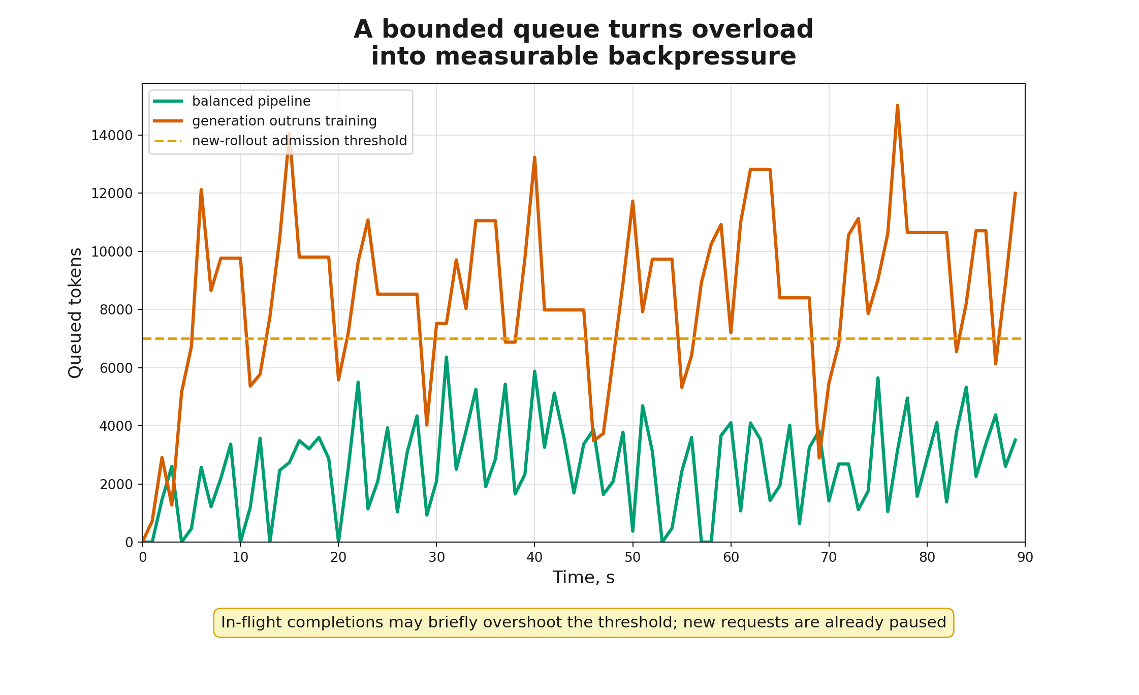
The module’s deterministic event simulator makes the trade-off visible. The 120-second smoke profile uses the same seed, eight rollout workers, 4096-token training batches, and one trainer in all three configurations. It is not a framework benchmark; it is a tested model of the queue contract.
| Profile | Training tokens/s | Mean lag, versions | Mean normalized ESS | Rejected rollouts | Backpressure time |
|---|---|---|---|---|---|
| sequential | 566.64 | 0.000 | 1.0000 | 0 | 0.0 s |
| bounded async, synchronize every update | 1442.38 | 1.803 | 0.9798 | 74 | 18.6 s |
| deeper overlap, synchronize every three updates | 1800.82 | 3.550 | 0.8804 | 0 | 52.8 s |
In this specific model, deeper overlap raises throughput while increasing lag and concentrating synthetic importance weights. The table does not define a universally optimal synchronization cadence; its coefficients were chosen to expose the mechanism. The defensible conclusion is narrower: throughput and freshness must be measured together.
The admission threshold applies to new work. It does not cancel requests already in flight, so observed queue depth may overshoot briefly as those requests finish. An implementation that does not state this rule can make a normal transient look like a broken counter.
Step 12.3.5 — Profile the timeline before interpreting GPU utilization
Average GPU utilization does not identify a bottleneck. Ninety percent may represent useful decode, weight conversion, or a stalled collective inside an active kernel.
A minimal profiling protocol is:
- assign one
trace_idacross prompt, rollout, and training batch; - record start and end of every stage;
- measure tokens as well as records;
- separate queue wait from compute time;
- record policy and verifier versions;
- measure after warm-up;
- report median and tail quantiles, not only the mean;
- change one parameter per experiment.
Useful stage names include:
queue_wait
prefill
decode
verifier
logprob_recompute
forward_backward
optimizer_step
weight_sync
checkpoint
The bottleneck is then identified from the critical path. If rollout is 70% of sequential time but already hidden behind training, faster decode may not change the period. If synchronization lies on every critical path, an ideal engine still cannot fix throughput.
The optional notebook builds a synthetic timeline and distinguishes total work, critical-path time, pool utilization, and steady-state throughput.
Lesson 12.4. Staleness, mismatch, and weight synchronization
Lesson 12.4. Staleness, mismatch, and weight synchronization
- Three policies and two different mismatches
- Probability ratios and effective sample size
- Identical weights do not guarantee identical probabilities
- What to do with stale data
- Weight synchronization must be atomic and measurable
then 4 assessment steps
Step 12.4.1 — Three policies and two different mismatches
Infrastructure discussions benefit from distinguishing three policies.
- The behavior policy actually sampled tokens in the rollout engine.
- The old policy is the frozen denominator of a PPO-like objective within an update.
- The current policy receives the gradient.
The token-level contract—causal shift, response masks, and the distinction among old, current, and reference log-probabilities—is constructed in RL for LLM, Module 6 “The LLM as a Policy: Tokens, Log-Probabilities, and KL” (rl_llm.module_06_llm_policy). Infrastructure does not alter those definitions; it must preserve them across serialization and process boundaries.
A separate reference policy may provide Kullback–Leibler (KL) regularization. It does not replace the behavior policy.
Now separate two failure modes.
Policy lag. Let denote the current published and trainable version, and let the rollout have been generated by version . The sample is stale when
Training–inference mismatch (TIM). Engine and trainer declare the same weight version but compute different probabilities because of:
- different numerical kernels or reduction order;
- precision or quantization differences;
- tensor-parallel layout;
- template, mask, or EOS differences;
- logit transformations used by decoding.
They require different diagnostics. Lag is measured by version and age. TIM is tested at zero lag: immediately after synchronization, score the same sequence in the engine and trainer and compare token log-probabilities.
A ratio far from one cannot be attributed automatically to staleness. Conversely, exact stack agreement does not remove version lag.
Step 12.4.2 — Probability ratios and effective sample size
For action in state , the importance ratio is
The ratio is defined only where the behavior policy assigns positive probability: . Full importance-sampling claims require support: the target policy must not assign positive probability to actions that the behavior policy could never produce. Numerical clipping cannot reconstruct missing support.
For a complete autoregressive sequence,
or, more stably,
Small token-level differences accumulate with length, so long completions are especially sensitive to lag and TIM.
For non-negative weights , effective sample size is
Equal weights give ESS ; one dominant record pushes it toward one. Normalized ESS, , compares batches of different sizes.
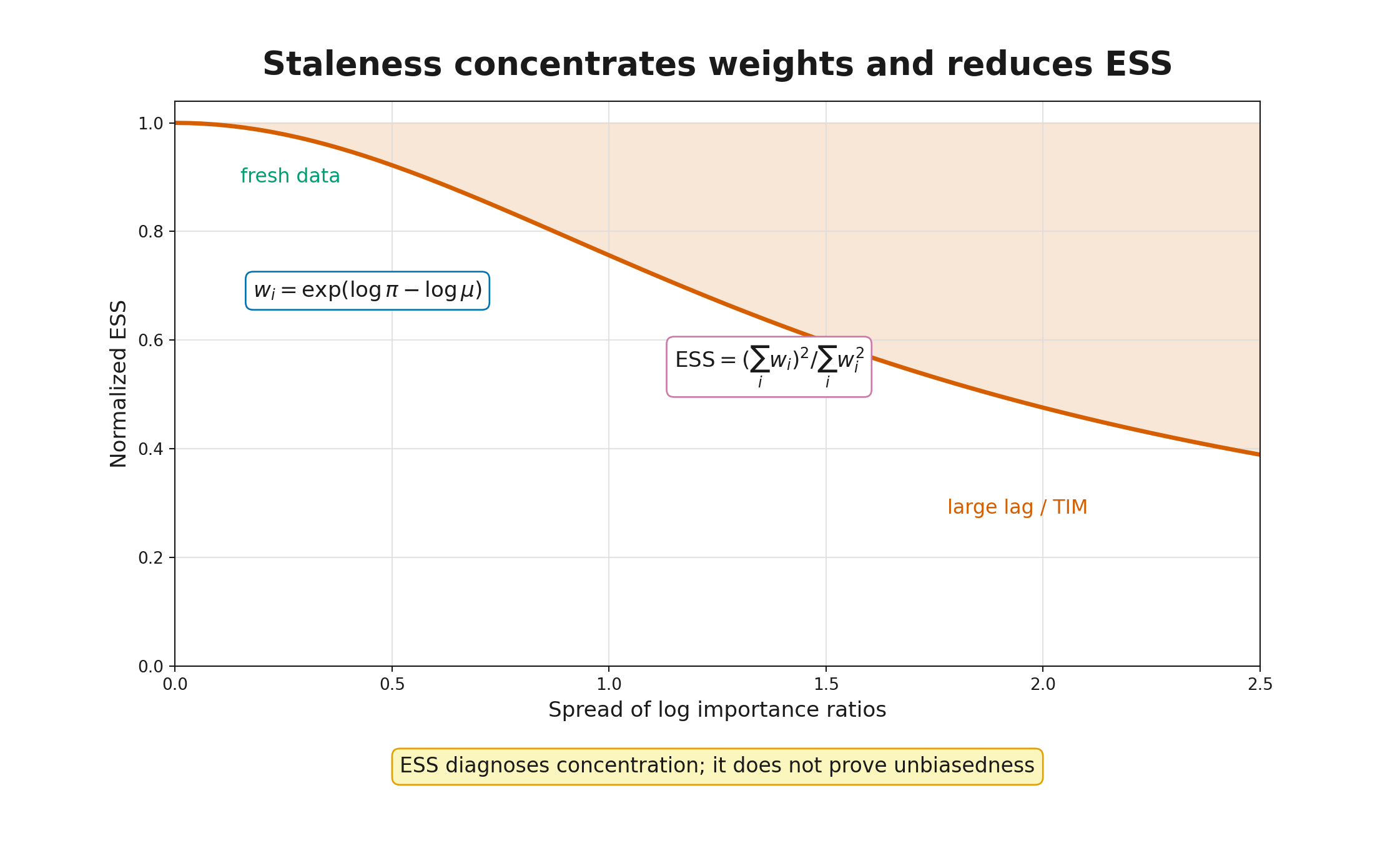
ESS is a concentration diagnostic, not proof of an unbiased update. Log policy lag, mean and maximum , clipping fraction, rejected records, gradient norm, and completion length together.
Step 12.4.3 — Identical weights do not guarantee identical probabilities
Suppose trainer and engine weights are byte-identical. It still need not follow that
Floating-point addition is non-associative. Batch shape, tensor parallelism, fused kernels, quantization, and softmax implementation can change logits slightly. For untruncated softmax, a uniform bound gives for every token; rarity alone does not amplify the relative change. Small differences can nevertheless accumulate across a long sequence, and crossing a top-k/top-p boundary changes the retained support.
Decoding is an even more direct source. If the engine applies top-p and renormalizes the retained set, the behavior log-probability is the probability after truncation. The untruncated softmax probability is not the behavior probability.
At the 2026-08-06 snapshot, official TRL documentation exposes a separate experimental Async GRPO path and vLLM integration, while verl documents corrections for rollouts produced by a different numerical stack or an older policy. These are implementation contracts, not universal rules of RL systems. Research on TIM reports that numerical mismatch can be an independent instability factor in studied configurations; this is an empirical warning, not proof that every run collapses.
Three practical regimes are:
- Recompute log-probabilities in the trainer. This is expensive but uses the same stack as the gradient.
- Store actual engine log-probabilities and apply an explicit correction. This requires a precise behavior policy and variance control.
- Unify kernels and configuration. This reduces mismatch but can restrict available optimizations.
The choice belongs in the experiment protocol.
Step 12.4.4 — What to do with stale data
Asynchrony does not make a rollout “wrong” automatically. It changes the statistical problem. Options include:
- impose a maximum lag ;
- reject records older than a threshold;
- use clipped or masked importance correction;
- reduce updates per rollout;
- lower the learning rate when ESS falls;
- rebalance pools so the queue stops growing;
- periodically return to a synchronous control run.
Each choice has a cost.
- Rejection improves freshness but wastes expensive rollouts and may favor short episodes.
- Clipping controls variance but changes the estimator.
- Full sequence ratios are natural for trajectory-level correction but become high variance on long responses.
- Token-level ratios are convenient and common but are not automatically equivalent to exact sequence correction under large lag.
AReaL and other asynchronous systems report speedups in their own configurations while introducing lag controls or specialized off-policy mechanisms. These results show that asynchrony can pay off; they do not define one universal safe lag.
Group advantages, clipping, and GRPO diagnostics are developed in RL for LLM, Module 9 “RLVR and GRPO: Verifiable Rewards, Group-Relative Estimates, and Stability” (rl_llm.module_09_rlvr_grpo). The systems-specific addition is that the lag distribution and queue policy determine which behavior policy belongs in the denominator.
A sound experimental order is:
- obtain a stable synchronous baseline;
- enable overlap with measured lag;
- measure ESS, clipping, and quality;
- deepen the queue only while statistical signal remains acceptable.
Step 12.4.5 — Weight synchronization must be atomic and measurable
New policy weights can reach the rollout engine through several paths.
- Full snapshot: gather, save or transfer, and reload the model. Simple but expensive in time and peak memory.
- Sharded transfer: convert an FSDP or Megatron layout directly to the engine layout and transmit shards through collectives.
- Adapter update: transfer only LoRA parameters when the engine and library support a consistent update path.
- Colocation: switch roles on the same GPUs and use a shared or convertible parameter representation.
Every path needs four properties.
- Version identifier. The engine reports the version it actually serves.
- Atomicity. A new request never sees a mixture of old and new tensors.
- Readiness barrier. The version is not considered available until all required replicas have loaded it.
- Verification. Tensor hashes or control logits confirm that the expected version is active.
Long requests should either finish under old weights or record the version of each action explicitly. Updating weights under a request and then assigning one version to the entire completion is invalid.
Current verl documentation describes checkpoint and weight transfer across training and rollout backends. OpenRLHF and NeMo RL document colocated or sleep/wake variants. Official vLLM documentation for NCCL weight transfer describes multi-node synchronization, a phased update protocol, and an asynchronous-generation example with mid-flight pause, weight synchronization, resume, and validation. These are mutable engineering contracts, not mandatory standards.
Lesson 12.5. Recovery, observability, and framework choice
Lesson 12.5. Recovery, observability, and framework choice
- An RL checkpoint is wider than model weights
- A trace must connect data to the update
- Recovery is tested by a failure, not by a directory
- Framework map at the 2026-08-06 snapshot
- Infrastructure is part of the algorithm
then 8 assessment steps
Step 12.5.1 — An RL checkpoint is wider than model weights
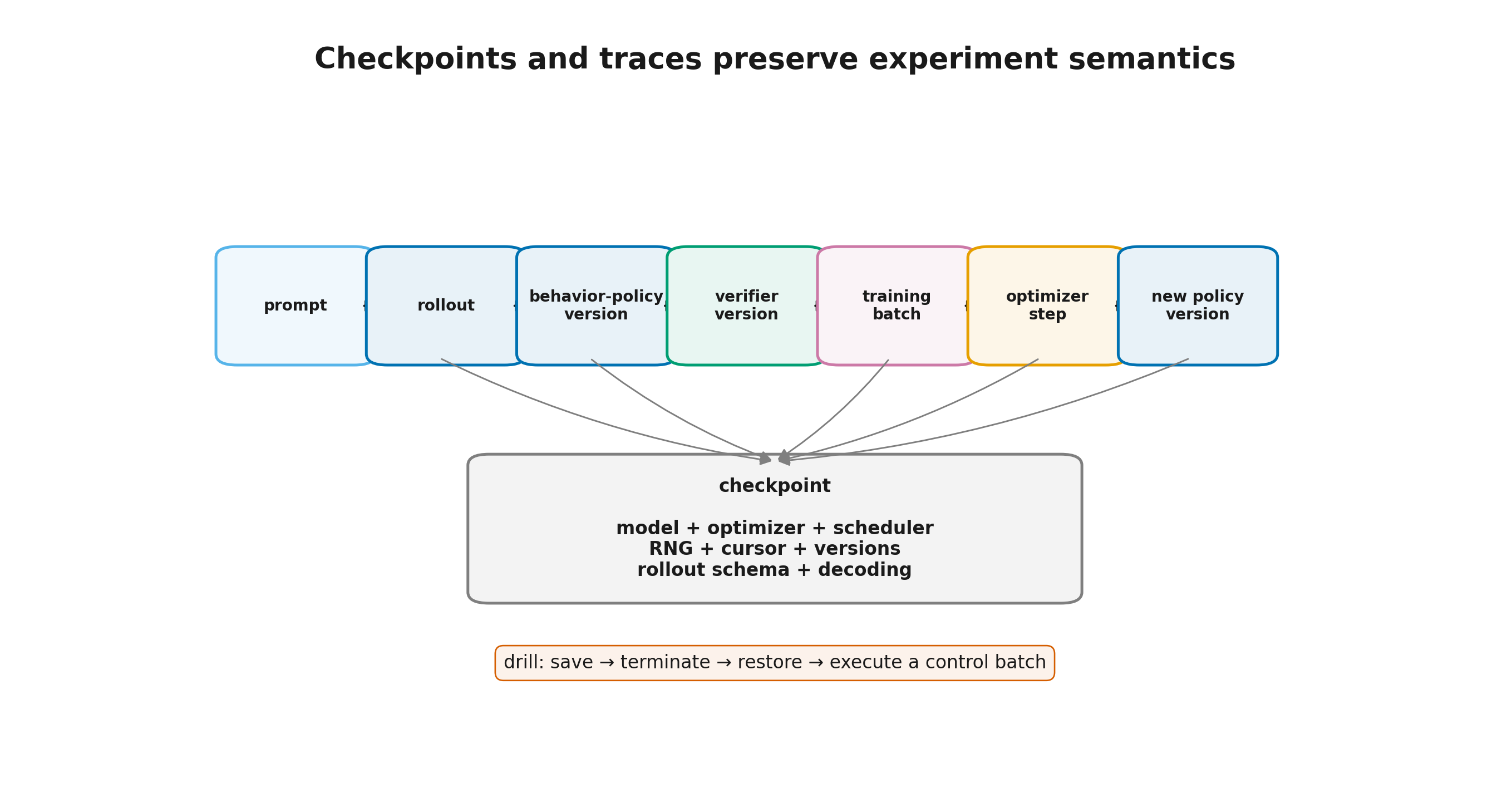
An honest restart requires more than policy parameters. A minimal checkpoint contains:
- model and adapter parameters;
- optimizer state;
- learning-rate scheduler;
- global step and policy version;
- random-number generator states;
- dataset cursor;
- curriculum or prompt-scheduler state;
- reward and advantage normalization;
- tokenizer, template, verifier, and environment versions;
- rollout schema;
- decoding configuration;
- distributed-layout metadata.
If a queue contains stale rollouts, recovery must either preserve it together with behavior versions or discard it explicitly. The same applies to unfinished agent episodes: save environment state or restart and mark them lost.
Engine weights do not necessarily need an independent checkpoint if they are deterministically reconstructed from the trainer checkpoint and synchronization recipe. The recipe—engine version, precision, quantization, and adapter conversion—still belongs in the manifest.
A simple failure model approximates checkpoint-writing and lost-work fraction by
where is checkpoint interval, is write time, and is mean time between failures. Its minimum is
This is an orientation tool, not a complete policy. Asynchronous writes, restart cost, and correlated failures alter the model.
Step 12.5.2 — A trace must connect data to the update
A dashboard says what changed; a trace says which events one record passed through.
The minimal identity chain is:
prompt_id
  -> rollout_id
  -> behavior_policy_version
  -> verifier_version
  -> training_batch_id
  -> optimizer_step
  -> resulting_policy_version
Useful metric families include:
Data
- prompt and completion length;
- stop reasons;
- infrastructure-error fraction;
- degenerate-group fraction;
- reward distributions.
Policy
- KL to the reference;
- entropy;
- log-probabilities and ratios;
- ESS;
- policy lag.
System
- stage-level tokens per second;
- queue wait;
- the 50th, 95th, and 99th percentiles of rollout duration (p50/p95/p99);
- pool utilization;
- synchronization time;
- peak memory;
- retries.
Reliability
- age of the latest successful checkpoint;
- save and restore time;
- lost rollouts;
- metric changes across restart.
A metric without configuration provenance is often misleading. Completion length changing after max_new_tokens changes is not spontaneous policy dynamics.
Step 12.5.3 — Recovery is tested by a failure, not by a directory
The existence of checkpoint-1000 does not show that training can continue. Recovery needs a routine drill.
- Run several steps and save a checkpoint.
- Record a configuration hash and a small metric baseline.
- Terminate one or more processes deliberately.
- Restore trainer, rollout engine, and scheduler.
- Restore or discard the queue according to the declared policy.
- Execute one control batch.
- Check finite losses, policy version, tokenization, and batch composition.
- Compare statistics against an allowed range.
Bitwise determinism is often too expensive or impossible after changing process count. The more practical goal is to preserve experiment semantics and avoid reporting a cold optimizer, reset curriculum, or changed verifier as a continuation of the same run.
Test at least three failures:
- one rollout worker dies;
- the trainer dies after writing a checkpoint;
- the verifier fails while a batch is only partially written.
A batch should be accepted as one complete transaction or rejected. A partial batch with unknown reward provenance must not silently enter training.
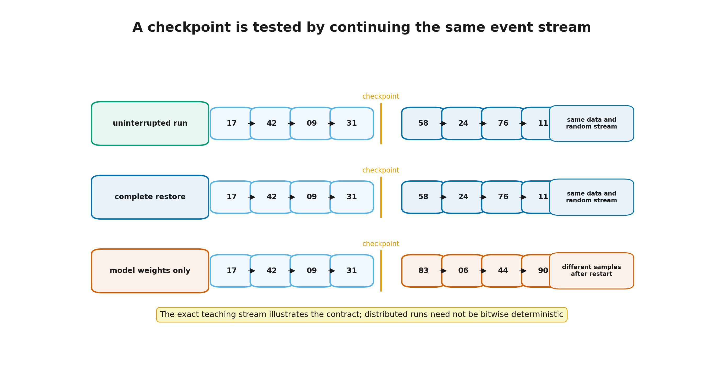
The notebook runs three branches of one teaching experiment. The uninterrupted branch and a full restore—RNG state, data cursor, and component versions included—produce the same event sequence. A weights-only restart diverges immediately. Exact equality is intentionally strict in this single-process example. A distributed run need not be bitwise deterministic, but it must preserve the declared experiment semantics and document acceptable sources of divergence.
Step 12.5.4 — Framework map at the 2026-08-06 snapshot
The following is a dated map, not a ranking. Features change quickly, so recheck the documentation and examples of the exact version before a run.
| Stack | Main abstraction level | Training | Rollout and placement | Asynchrony and agents | Practical profile |
|---|---|---|---|---|---|
| TRL | ready-made trainers around Transformers | Accelerate, DeepSpeed, and related integrations | vLLM colocate or server modes | experimental Async GRPO and environment integrations in current docs | fast research route and small or medium runs |
| verl | programmable HybridFlow RL dataflow | FSDP/DTensor and Megatron paths | vLLM or SGLang; colocated and disaggregated layouts | fully asynchronous and one-step-off recipes, agent loop, checkpoint engine, and rollout correction | flexible large-scale system with explicit version control |
| OpenRLHF | Ray orchestration of roles | DeepSpeed ZeRO | vLLM and a hybrid engine | asynchronous training, partial rollouts, and an agent interface in the current release | distributed RLHF/RLVR recipes |
| NeMo RL | NVIDIA distributed post-training recipes | DTensor or Megatron Core | vLLM and several generation paths | documented Async GRPO with importance correction and environment integrations | large runs in the NVIDIA ecosystem |
| PRIME-RL | fully asynchronous dataflow as described by the project | FSDP2 and specialized paths | vLLM with disaggregated generation | emphasis on fully asynchronous and long-running training | modern engineering stack; project claims need local reproduction |
| SkyRL | modular full-stack system | project-supported distributed backends | vLLM and a unified training/rollout interface | agent layer and asynchronous dispatch | reasoning and multi-turn research |
| AReaL | research-oriented fully asynchronous system | its distributed trainer | streaming rollout workers | explicit lag control and off-policy mechanisms | studying benefits and risks of full asynchrony |
HybridFlow describes RLHF as a distributed dataflow in which each logical model is a program, with layout conversion between training and generation. The official verl fully asynchronous recipe reports author-measured 2.35–2.67× speedups for stated Qwen2.5-7B configurations on 128 GPUs; AReaL reports up to 2.57× over its compared synchronous systems. These are author-protocol results, not guarantees for another cluster, model, or length distribution.
Framework selection begins with requirements:
- one node or many;
- full fine-tuning or LoRA;
- one-shot or multi-turn rollouts;
- synchrony, allowed lag, and queue policy;
- FSDP, Megatron, or DeepSpeed;
- vLLM or SGLang;
- recovery and telemetry requirements;
- the team’s ability to debug the chosen abstraction level.
Step 12.5.5 — Infrastructure is part of the algorithm
The module now forms one continuous chain.
- The behavior policy samples tokens under a concrete weight version and decoding rule.
- The rollout stores tokens, masks, log-probabilities, reward, stop reasons, and component versions.
- The queue bounds age, volume, and cost.
- The trainer updates relative to the declared behavior policy and monitors probability ratios.
- Synchronization atomically publishes a new version.
- A checkpoint preserves enough state to continue the same experiment.
- A trace connects an individual completion to an optimizer step and back.
The central conclusion is:
In online RL, infrastructure determines not only compute speed but also the statistical meaning of data. Queues, weight versions, decoding, and synchronization are part of the algorithm specification.
A conservative progression for a large run is:
- establish a one-process sequential baseline;
- validate the rollout contract and zero-lag log-probabilities;
- build a component- and phase-level memory ledger;
- measure critical paths and tail latency;
- add overlap before full asynchrony;
- log lag, TIM, ESS, and clipping fraction;
- test recovery with an injected failure;
- compare stacks on the same task and cost units.
The next and final theory module is RL for LLM, Module 13 “Evaluating RL Systems for LLMs: Statistics, Reward Hacking, and Safety” (rl_llm.module_13_evaluation). The infrastructure contract established here tells us where data came from; Module 13 asks whether conclusions drawn from those data can be trusted.
Sources and further reading
The following primary papers and official documents support the module’s most consequential claims. The full claim-by-claim registry, including evidence class, access date, and limits of each inference, is in Module_12_Sources.md.
- ZeRO: Memory Optimizations Toward Training Trillion Parameter Models — the primary account of staged model-state partitioning; it does not replace an activation and temporary-buffer trace for a concrete run.
- Efficient Memory Management for Large Language Model Serving with PagedAttention — the primary PagedAttention and vLLM paper; reported speedups belong to the paper’s configurations.
- SGLang: Efficient Execution of Structured Language Model Programs — the source for RadixAttention and prefix reuse.
- HybridFlow / verl and the official fully asynchronous recipe — distributed RL dataflow and dated author-reported asynchronous results.
- AReaL: A Large-Scale Asynchronous Reinforcement Learning System for Language Reasoning — a primary fully asynchronous RL system paper with explicit lag control; numerical gains are author reports.
- Diagnosing Training–Inference Mismatch in LLM Reinforcement Learning — analysis of probability mismatch between rollout and training stacks; it does not imply that every kernel difference necessarily destabilizes training.
- TRL: Asynchronous GRPO, verl: rollout correction, NeMo RL: Async GRPO, OpenRLHF: RL training, and vLLM: NCCL weight transfer — mutable software contracts checked at the 2026-08-06 snapshot; pin resolved versions before execution.
- A First Order Approximation to the Optimum Checkpoint Interval — the source of the teaching Young interval; correlated failures and tiered storage require richer models.