Module 2. State, Value, and Bellman Equations
Material version: 2026.7
Content snapshot: 2026-08-04
Language: EN
Core practice: Tier A — browser, Python, NumPy, and a central processing unit (CPU)
Structure: 4 lessons, 20 steps
Estimated time: 8–12 hours including the core lab
Module 1 framed RL as a loop of action selection and feedback. We now face a harder question: how can we evaluate a state or an action before the final outcome is known? The answer begins with a well-chosen state representation, continues with value functions, and leads to the Bellman equations.
A prior classical RL course is still not required. New concepts are introduced in plain language, formalized, and only then mapped to LLMs. Readers who already know RL can move quickly through §§2.1.1–2.1.4 and focus on the limits of the token-level model, termination versus truncation, the exact conditions behind convergence statements, and the bridges to modern LLM post-training.
Learning goals. By the end of the module, you will be able to:
- check whether a state representation contains enough information for a Markov model;
- distinguish a state from an observation and task termination from technical trajectory truncation;
- compute , , and the advantage , and interpret them for LLM generation;
- derive the Bellman expectation equation from the return recursion;
- solve a small tabular decision process as a linear system or by iteration;
- distinguish Monte Carlo evaluation, one-step temporal-difference learning, and -step targets;
- explain two tabular control methods through behavior and target policies;
- recognize maximization bias and explain how separating selection from evaluation reduces it;
- reproduce numerical experiments on Gridworld, FrozenLake, the Corridor, and CliffWalking.
The public computational lab is the executable practice. It implements exact policy evaluation, value iteration, Monte Carlo prediction, TD(0), multi-step TD, Q-learning, SARSA, and Double Q-learning. NumPy, Matplotlib, and a CPU are sufficient; no GPU is required.
Practice route. Graded tasks, worked solutions revealed after an attempt, and executable practice follow the lecture. The explanation remains self-contained.
Lesson 2.1. From history to state, then to value
Lesson 2.1. From history to state, then to value
- Why we need a state
- A finite MDP and the reward convention
- Task termination and technical truncation are different
- Three value functions: V, Q, and advantage A
- Reading value functions for an LLM
then 7 assessment steps
Step 2.1.1 — Why we need a state
The complete interaction history at time may be long:
The word state is used for two related but distinct objects.
- An environment state is a variable relative to which future dynamics are Markov. It need not be a compression of anything the agent has observed.
- An agent state or representation is constructed from available history: a transcript, a finite window, recurrent memory, or an external-memory record. It is only a candidate sufficient state.
Let be the chosen representation. It is one-step sufficient when
This equation does not claim that the world has forgotten its past. It says that, once and are fixed, earlier history should not further change the conditional distribution of the next state and reward.
Three questions, not one. What does the environment actually store? What can the agent observe? What internal record does the agent use to choose an action? Simple textbook tasks make the three coincide; tool-using systems often do not.
An observation may be incomplete. A sufficient state supports a Markov decision process (MDP). When hidden environment variables affect future transitions, a partially observable Markov decision process (POMDP) is the natural model, and the agent may rely on observation history, memory, or a belief over hidden state.
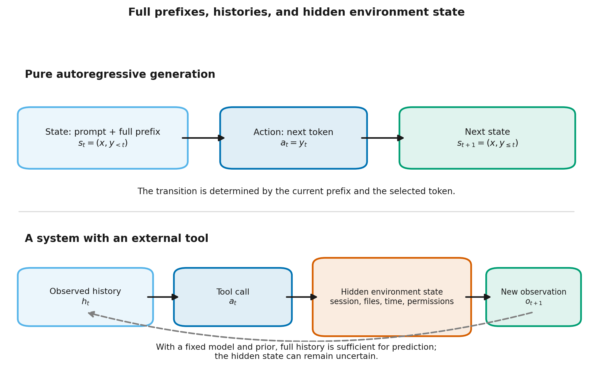
For pure autoregressive generation, one may write
If the transition only appends the chosen token, model parameters and decoding rules are fixed, and stopping depends on the visible prefix, the complete prefix is sufficient. Random token sampling is not a violation: it belongs to the policy , while the transition to the next prefix is deterministic once the token action has been fixed.
A browser, file session, user, or external tool can carry hidden state. For a fixed environment model and initial distribution, the complete history can serve as a growing information state: it determines the conditional distribution of future observations and rewards without revealing the actual world state. The belief summarizes that history for prediction in a POMDP. Different hidden states compatible with one history can produce different outcomes while belonging to the same conditional probability law.
A text-message window may contain only part of . For example, the message identifying the open file may have been dropped, while the file session still uses that file. Two complete histories then produce the same window even though their earlier observations change the prediction of the next tool response. The loss of relevant information in the representation, rather than hidden state alone, makes that window insufficient.
Practical sufficiency test. Can two complete histories mapped to the same record give different conditional distributions of the next observation and reward under the same action? If so, the representation has lost relevant information. Different random outcomes drawn from one conditional distribution do not violate the Markov property.
Architecture context: Modern LLMs, Module 18 “Agents and Tool Use” (modern_llms.module_16_agents) develops the systems view. Here we only need the distinction among environment state, observation, and the agent's internal representation.
Step 2.1.2 — A finite MDP and the reward convention
We define a finite MDP by
Here:
- is the state space;
- is the action space;
- is the next-state distribution;
- is the reward distribution on a transition;
- is the initial-state distribution;
- is the discount factor.
Tabular calculations often store the conditional mean reward rather than the full reward distribution:
The expected reward always exists when the reward is integrable and satisfies . This marginalization requires no conditional-independence assumption. Equating with the same for every reachable next state is an additional assumption about the conditional mean. Likewise, can average over actions under a specified policy, whereas an action-independent reward model is a stronger condition. This module uses the transition-conditioned form by default.
The policy is not part of the environment dynamics. The same MDP can be paired with different policies. Under a fixed policy, a one-step joint distribution factors as
This factorization will soon become the Bellman equation: average over policy actions, then over environment transitions and rewards.
An episodic task reaches a terminal state. A continuing task may have no natural terminal state; for an infinite horizon, one commonly uses or another objective that remains finite.
Throughout this module, reward belongs to a transition. If entering the goal pays , that reward remains in even though . Zero terminal value removes future continuation; it does not erase the final reward.
Step 2.1.3 — Task termination and technical truncation are different
A trajectory file may record the same surface fact—“there is no next sample”—for two mathematically different reasons.
- Termination means the task itself reached a terminal state: success, failure, or an answer-ending token. The specified MDP has no continuation after that transition.
- Truncation means collection stopped because of an external budget: steps, wall-clock time, buffer capacity, or batch length. The underlying task could have continued.
Define a continuation mask
A one-step target becomes
or, equivalently,
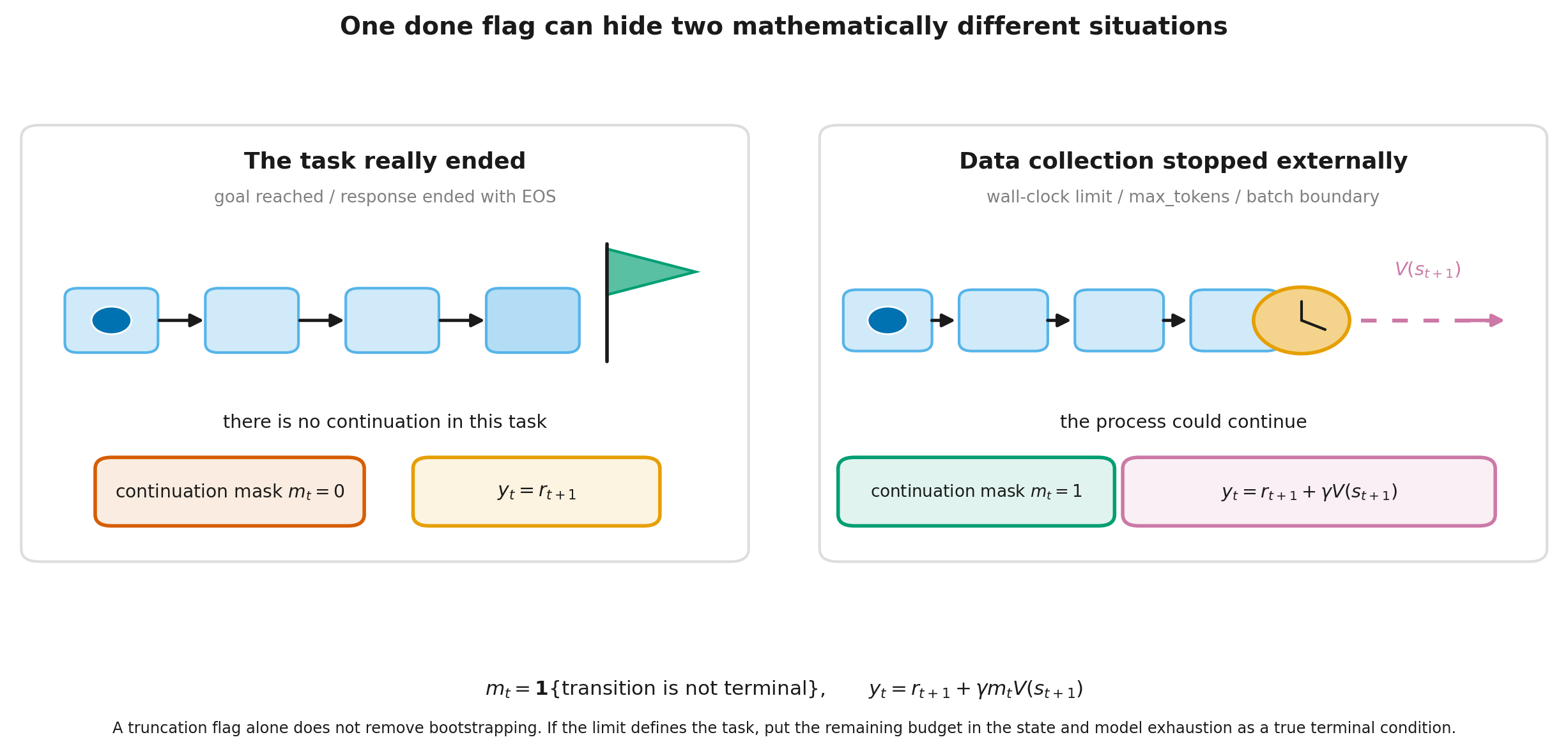
When a time limit defines the task, remaining time belongs in state and exhausting it may be a true terminal outcome. When the limit exists only for data collection, zeroing continuation is usually wrong.
For LLM systems:
- an end-of-sequence (EOS) token usually represents answer termination;
max_tokensis often truncation when a longer completion would still be meaningful;- “answer within 256 tokens” makes the same budget part of the objective;
- stopping a rollout because a batch is full is infrastructure, not task completion.
Conflating the cases creates systematic bias. With positive continuation value, treating truncation as terminal pushes the target down; with negative continuation value, it pushes the target up. Gymnasium therefore exposes terminated and truncated separately. Two flags do not remove the modeling decision: the environment author must still decide whether a limit belongs to the task.
Step 2.1.4 — Three value functions: V, Q, and advantage A
Fix a policy and define the return
for a continuing task, or the corresponding finite sum for an episode.
The state-value function is the expected outcome when starting from state and following the policy:
The action-value function fixes the first action and follows the policy afterward:
Therefore the state value is the policy-weighted average of the action values:
The advantage function compares an action with the current policy's average behavior:
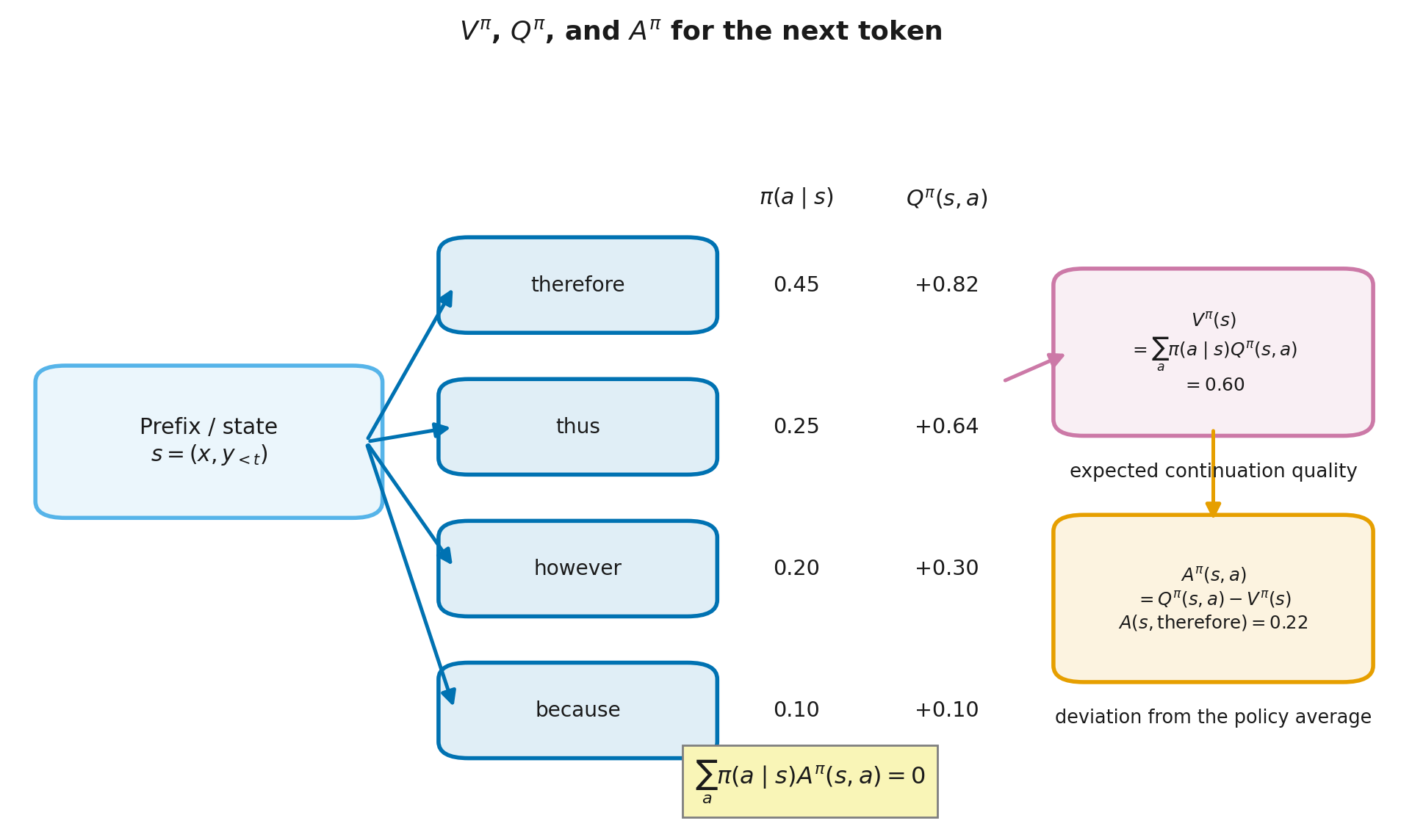
The definition immediately implies
A positive means “better than the current policy's average action in this state,” not “objectively good under every policy.”
A useful invariance is also immediate. Add the same constant to all action values in a state. The recomputed state value shifts by the same amount and the advantages stay unchanged:
This is a statement about shifting action-value estimates within a fixed state. It does not imply that an arbitrary change to the reward function leaves advantages unchanged throughout an MDP.
Under the transition-reward convention, . A final episode or response score is paid on the transition into that terminal and is already part of .
Step 2.1.5 — Reading value functions for an LLM
In a token-level model, state is the prompt plus generated prefix and action is the next token. Then
- is expected final reward after fixing token now and continuing under ;
- is the policy average over possible next-token choices;
- measures the token's deviation from that current-policy average.
A tiny prefix tree makes the definitions concrete. Suppose the prefix “because” leads to “check” with probability and reward , or to “skip” with probability and reward . Then
If the alternative prefix “guess” has value , and the empty prefix chooses “because” with probability , then
The notebook computes exactly this tree. It is not a miniature claim about real LLM scale; it isolates what token-level means: fix one next token, then average every continuation that follows under the policy.
Real value estimation is difficult. Prefix spaces are enormous, final reward often arrives only after a complete response, and nearly identical reasoning traces may receive different evaluations. Neural RL therefore uses learned critics, process evaluators, continuation predictors, or algorithms without a separately trained critic.
A common overreach concerns group relative policy optimization (GRPO). In the original DeepSeekMath construction, several complete responses are sampled for one prompt and their rewards are normalized within the group. This supplies a relative signal without a learned value model. The finite-group statistic is nevertheless a response-level sample baseline, not an exact at every token prefix. Later GRPO variants alter normalization, aggregation, and token assignment, so the method name alone does not specify every detail.
The bridge worth keeping. A value function asks what an unseen continuation is worth in expectation. A PPO critic, a GRPO group baseline, and a partial-reasoning evaluator approximate that broad question in different ways; they are not the same mathematical object.
Module 4 (rl_llm.module_04_policy_gradients) will connect advantage to policy gradients and GAE. Module 9 (rl_llm.module_09_rlvr_grpo) develops GRPO variants. Module 15 “Reasoning Models and Test-Time Compute” in Modern LLMs (modern_llms.module_13_reasoning) supplies the architectural context for scoring intermediate steps.
Lesson 2.2. Bellman equations: evaluation and improvement
Lesson 2.2. Bellman equations: evaluation and improvement
- One-step decomposition of the return
- Exact policy evaluation as a linear system
- Optimality and the exact contraction condition
- Evaluation, improvement, and generalized policy iteration
- Reproducible example: FrozenLake
then 6 assessment steps
Step 2.2.1 — One-step decomposition of the return
Module 1 gave us the return recursion
Take the conditional expectation at under a fixed policy :
Terminal states may remain in the sum when their continuation values are defined as zero. Reward paid on entry remains in .
In words:
state value is expected immediate reward plus discounted continuation value, averaged over the policy's action and the environment's transition.
For action value, the first action is already fixed:
Define the fixed-policy Bellman operator
The true value is its fixed point:
An operator is simply a rule that maps an entire value vector to a new one-step-backed-up vector.
What Bellman consistency does not specify. It does not choose a data source, a function class, or an optimizer, and it does not guarantee that neural training will reach the fixed point. Different exact and approximate algorithms are built from the same consistency relation.
Step 2.2.2 — Exact policy evaluation as a linear system
For a fixed policy, combine the action choice into
The Bellman equation becomes
so
For a finite discounted MDP with , is invertible and the solution is unique. At , the generic discount-based guarantee disappears. An episodic problem can still be solved over non-terminal states when the fixed policy reaches a terminal state almost surely and the resulting matrix is nonsingular.
A classic grid has terminal states in the upper-left and lower-right corners, reward per move, and an equiprobable random policy. Its exact value function for is
The entries are the negative expected numbers of steps to a terminal state under the random policy.
For an approximate value function , define the Bellman residual
A zero residual solves the equation exactly. For ,
Thus a small one-step residual can still correspond to a noticeable long-horizon error when is close to one.
Step 2.2.3 — Optimality and the exact contraction condition
Policy evaluation asks, “how good is this fixed policy?” Control asks, “which action should be selected?”
The optimal value function satisfies
Define the optimality operator
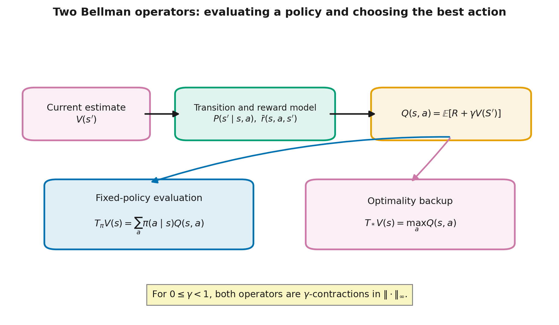
For , both operators are -contractions in the max norm. The key step for is
Taking the maximum over states gives
This gives a unique fixed point and geometric convergence of .
The boundary matters. At , the contraction factor is one, so this proof no longer establishes convergence. Some finite episodic problems at are still well posed and admit convergent dynamic-programming schemes, but they require additional assumptions. In a stochastic-shortest-path formulation, for example, there must be a policy that reaches a terminal state from every relevant state almost surely in finite expected time, and non-terminating policies cannot be allowed to remain competitive as though they had an ordinary finite cost. Merely adding a terminal state is not enough. “The Bellman operator is always a strict contraction” is false without a regime qualifier.
Step 2.2.4 — Evaluation, improvement, and generalized policy iteration
The Bellman equations suggest two alternating operations.
- Policy evaluation: approximate for the current .
- Policy improvement: select actions that maximize the one-step estimate
Evaluating to convergence and then improving greedily gives policy iteration. Maximizing on every sweep gives value iteration:
The broader pattern is generalized policy iteration (GPI): evaluation and improvement may be partial, asynchronous, and performed on different timescales, while each operation pushes the other toward consistency.
| Method | What is fixed inside the update | Result at convergence |
|---|---|---|
| Iterative evaluation | policy | |
| Policy iteration | full evaluation, then greedy improvement | an optimal policy |
| Value iteration | maximization on every one-step backup | and a greedy policy |
GPI is not a single algorithm with one formula. It is a pattern. In actor–critic methods, the critic evaluates while the actor improves. Tabular control exposes the same two operations without neural networks or optimizers.
Step 2.2.5 — Reproducible example: FrozenLake
module_2_reference.py contains a self-contained NumPy version of slippery FrozenLake. For each intended direction, the intended move and two lateral deviations have probability . Holes and the goal are terminal, and reward is paid only on entry to the goal.
Let be the number of transitions until the episode ends, either in the goal or a hole. Because reward is emitted only on entry to the goal, a successful trajectory contributes to , while an unsuccessful one contributes zero. Under optimal behavior,
With , value is therefore not a bare success probability: earlier success receives more weight.
from module_2_reference import build_frozen_lake_4x4, value_iteration

P, R, terminal = build_frozen_lake_4x4()
V, sweeps = value_iteration(P, R, gamma=0.9, terminals=terminal)
print(sweeps)
print(V.reshape(4, 4))
Starting from zero, synchronous value iteration with tolerance takes 145 complete sweeps and returns
[[0.068891 0.061415 0.074410 0.055807]
 [0.091855 0.000000 0.112208 0.000000]
 [0.145436 0.247497 0.299618 0.000000]
 [0.000000 0.379936 0.639020 0.000000]]
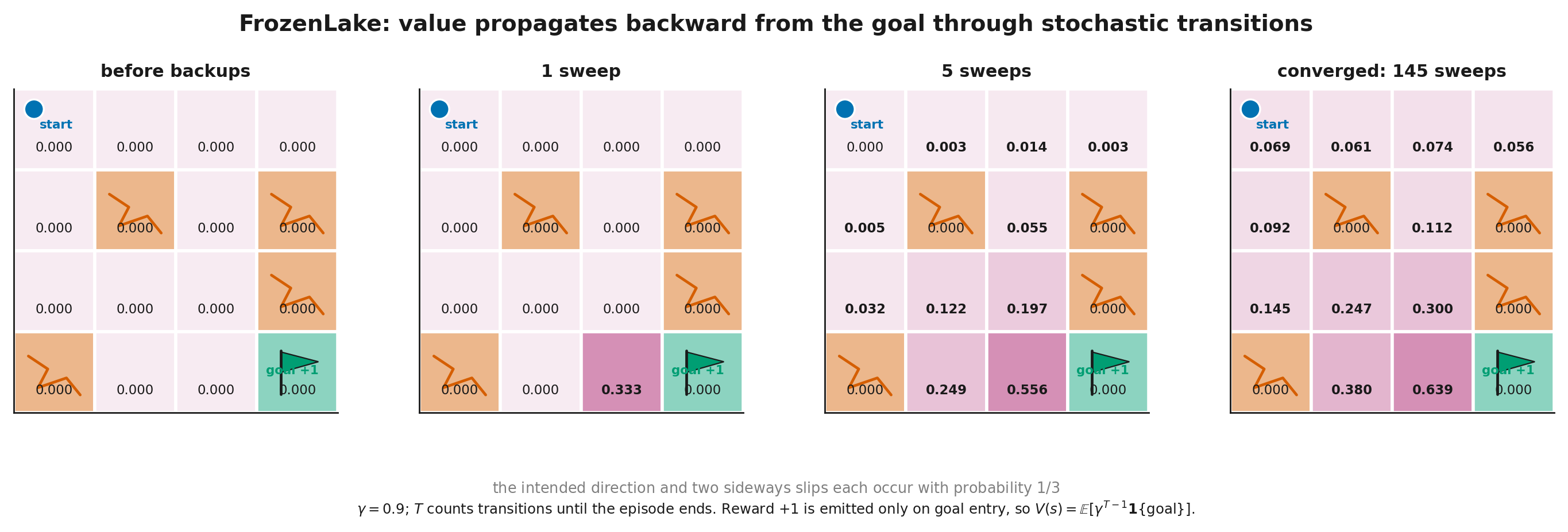
After one sweep, value is nonzero only where the goal can be entered in one transition. Later sweeps carry the signal backward through stochastic dynamics. Nothing physical is “flowing” through the grid; the picture shows repeated application of a one-step operator to an improving continuation estimate.
The number 145 belongs to this exact protocol: dynamics, action indexing, , zero initialization, synchronous updates, and stopping tolerance. Change any of them and the sweep count may change.
The tabular example matters for an LLM course because it exposes three durable ideas:
- a one-step target links the present estimate to continuation value;
- evaluation and improvement form a feedback loop;
- continuation error propagates over the horizon.
Neural approximation removes the simple tabular guarantees. Data distribution, optimization, architecture, and jointly changing parameters now matter. The Bellman equation remains a target relation, not an automatic convergence certificate.
Lesson 2.3. Model-free prediction: from full trajectories to bootstrapping
Lesson 2.3. Model-free prediction: from full trajectories to bootstrapping
- Prediction from sampled trajectories
- Monte Carlo evaluation
- One observed step and a continuation estimate
- A multi-step target connects MC and TD
- The Corridor: compare estimators, not slogans
then 6 assessment steps
Step 2.3.1 — Prediction from sampled trajectories
So far, and were known. In an actual environment, an agent usually sees only sampled transitions
The prediction problem estimates or for a fixed policy from interaction data without an explicit dynamics table.
Such a method chooses a target and moves the current estimate toward it. For tabular ,
where is the step size. The main difference among methods is the choice of .
- A full observed return barely depends on the current estimate, but requires waiting for the episode tail.
- A one-step target is available immediately, but uses the imperfect estimate .
- Intermediate -step targets consume several observed rewards and then bootstrap.
Bootstrapping means updating one estimate from another current estimate. It is unrelated to the statistical bootstrap based on resampling.
Step 2.3.2 — Monte Carlo evaluation
A Monte Carlo (MC) method uses the observed return itself:
For first visits to state , one may average all subsequent returns:
When episodes truly come from a fixed policy, termination is handled correctly, and returns have finite expectation, this is an ordinary sample mean whose expectation is . In this restricted sense, the MC target does not contain bias from the current continuation estimate.
That does not make every practical MC estimator automatically unbiased. Technical truncation, a changing policy, constant step sizes, initialization, and dependent data reuse can alter its statistical properties.
Strengths:
- no transition model is required;
- there is no bootstrapping;
- current value-estimation error is absent from the target.
Limitations:
- enough of the trajectory, often the whole episode, must be observed;
- a single terminal reward may produce high variance;
- long episodes are expensive;
- rarely visited states accumulate data slowly.
A full LLM response with one final score is an MC-like sequence-level signal: the outcome is observed after generation, but the contribution of each token remains hidden.
Step 2.3.3 — One observed step and a continuation estimate
Temporal-difference learning (TD) updates before an episode ends. The one-step TD(0) target is
for a non-terminal transition. The temporal-difference error is
The update is
At a true terminal state, the continuation is zero:
At a technical truncation where the process could continue, is normally retained.
TD(0) uses fewer random future rewards but relies on the current estimate. Its finite-sample target therefore inherits value-estimation error. This often reduces variance at the cost of bias, but there is no universal ordering in which TD always beats MC or vice versa. The outcome depends on the environment, representation, step size, and data budget.
A useful intuition: MC waits for the bill for the whole route; TD revises the current estimate after each newly observed segment.
Step 2.3.4 — A multi-step target connects MC and TD
If the task does not terminate within the next transitions, the -step target is
At this is TD(0). If a true terminal occurs before the end of the window, the observed sum stops at that transition and no continuation term is added. When the window covers the remaining episode, the target becomes Monte Carlo.
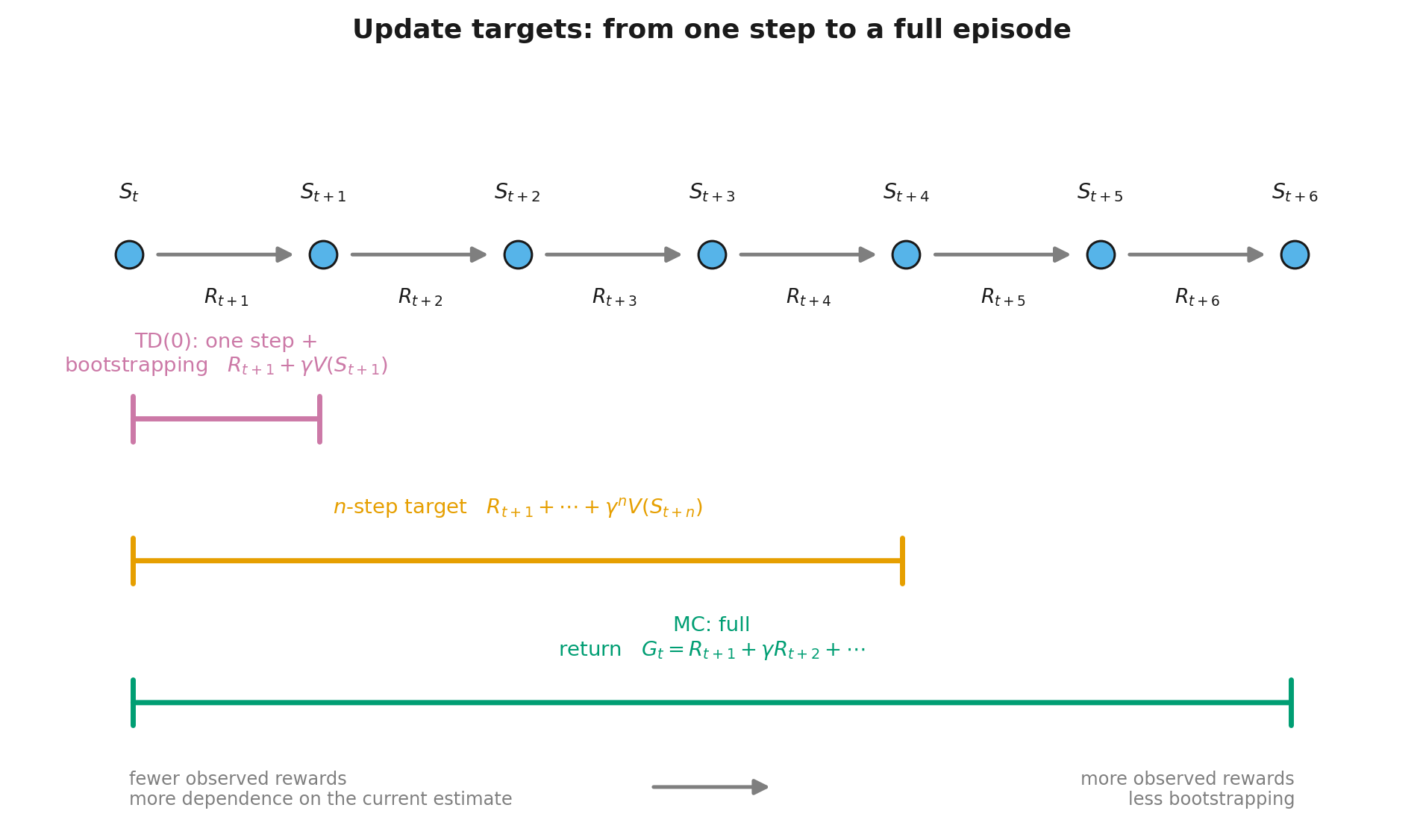
Increasing usually means
- more observed reward in the target;
- less dependence on the current estimate;
- a longer wait before updating;
- more exposure to randomness in a longer trajectory segment.
Those tendencies are not a monotone quality guarantee. Representation error, step size, temporal correlation, and episode length can change the best horizon.
Generalized advantage estimation (GAE) will later combine temporal-difference residuals across horizons with exponential weights. The important precursor is already here: an -step target chooses where observed trajectory data give way to a current continuation estimate.
The reference n_step_target() receives observed rewards, a bootstrap value, , and an explicit terminal flag for the end of the window. That interface prevents external truncation from being silently treated as task termination.
Step 2.3.5 — The Corridor: compare estimators, not slogans
Consider a symmetric five-cell Corridor with terminals at 0 and 4, a middle start, and equal-probability left/right actions. Reward is paid only on entry to the right terminal. At , the values are the probabilities of reaching the right side before the left:
The figure uses one controlled protocol:
- episode budgets from 20 to 2,500;
- 40 independent random seeds;
- first-visit Monte Carlo;
- TD(0) and three-step TD with constant ;
- root mean squared error (RMSE) over the three non-terminal states;
- a median line and interquartile band.
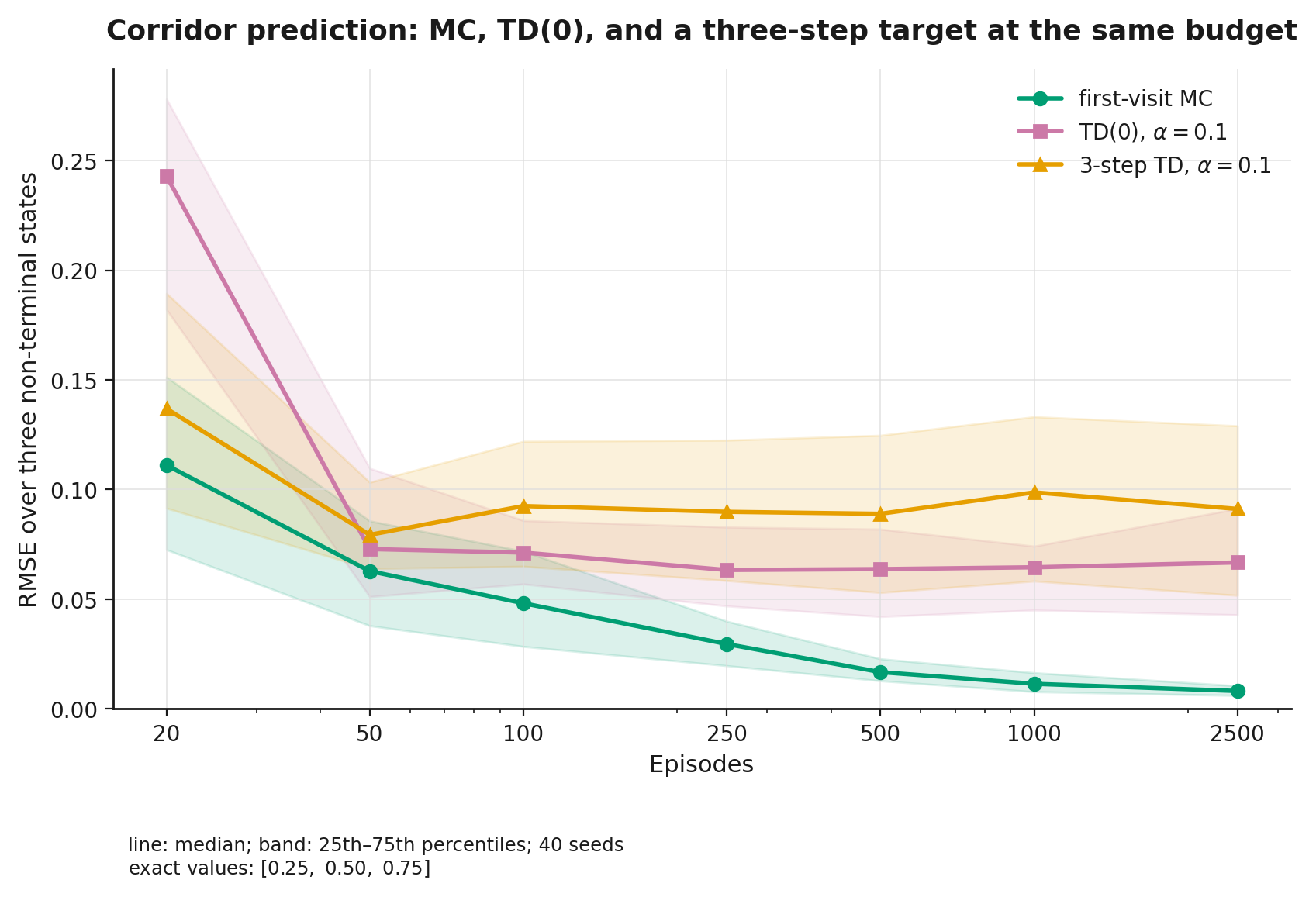
The experiment is designed to resist a universal slogan. At small budgets, noise and initialization dominate. With more data, the MC sample mean continues toward the exact value. Constant-step-size TD retains residual variation. Three-step TD is not guaranteed to sit between the other curves at every budget; it follows its own interaction between observed rewards and current estimates.
Reference outputs include
exact: [0.00, 0.25, 0.50, 0.75, 0.00]
MC, 1000 episodes, seed=7:
       [0.00, 0.255539, 0.496000, 0.733728, 0.00]
TD(0), 1000 episodes, seed=42, alpha=0.1:
       [0.00, 0.233105, 0.582660, 0.829850, 0.00]
3-step TD, 1000 episodes, seed=42, alpha=0.1:
       [0.00, 0.248712, 0.523243, 0.769480, 0.00]
The different seeds in these lines are reproducibility fixtures, not a contest. Annealed step sizes, another horizon, function approximation, reused data, or non-stationarity would change the result.
LLM bridge. A final score on a complete response resembles an MC observation. A critic, process evaluator, or continuation predictor introduces bootstrapping. Group normalization compares complete responses but does not by itself become an exact token-level value function.
Lesson 2.4. Control: behavior and target policies
Lesson 2.4. Control: behavior and target policies
- From fixed-policy prediction to behavior improvement
- Two update targets differ by one line, not by one detail
- CliffWalking: one protocol, different routes
- Why a maximum overestimates noisy values
- What transfers to LLM RL, and what remains a tabular teaching model
then 6 assessment steps
Step 2.4.1 — From fixed-policy prediction to behavior improvement
In control, the policy changes during learning. It helps to distinguish:
- the behavior policy, which actually selects actions and collects data;
- the target policy, whose value is being estimated or improved.
When they match, learning is on-policy. When they differ, learning is off-policy. These labels are not defined by the presence of a replay buffer or by random exploration itself; they describe which policy is inferred from which policy's data.
A simple exploration rule is -greedy:
- with probability , choose an action maximizing ;
- with probability , choose a random action.
This prevents the learner from immediately locking onto its first apparent route. Systematic exploration is the subject of Module 3; here lets us expose the difference between two update targets.
Step 2.4.2 — Two update targets differ by one line, not by one detail
Both methods update tabular :
The state–action–reward–state–action method (SARSA) uses the next action actually selected by the behavior policy:
With -greedy behavior, SARSA evaluates the consequences of future exploration. It is on-policy.
Q-learning uses a greedy target regardless of the action that will actually be executed next:
Data may be gathered by an -greedy behavior policy, while the target refers to the greedy policy. Q-learning is therefore off-policy.
At a terminal transition, both targets reduce to . At a technical truncation, the continuation is normally retained.
In a finite discounted tabular MDP with bounded rewards, classical Q-learning convergence requires every state–action pair to be visited infinitely often and, for each pair, step sizes satisfying and . This is an asymptotic tabular stochastic-approximation result. Constant step size, finite data, neural functions, changing targets, and jointly trained components do not inherit it automatically.
Step 2.4.3 — CliffWalking: one protocol, different routes
In CliffWalking, the agent moves from the lower-left to the lower-right corner. An ordinary step yields . Entering the cliff yields and returns the agent to the start. Behavior remains -greedy during training.
The static figure uses
- random seed 0;
- 500 episodes;
- ;
- ;
- ;
- greedy evaluation after training.
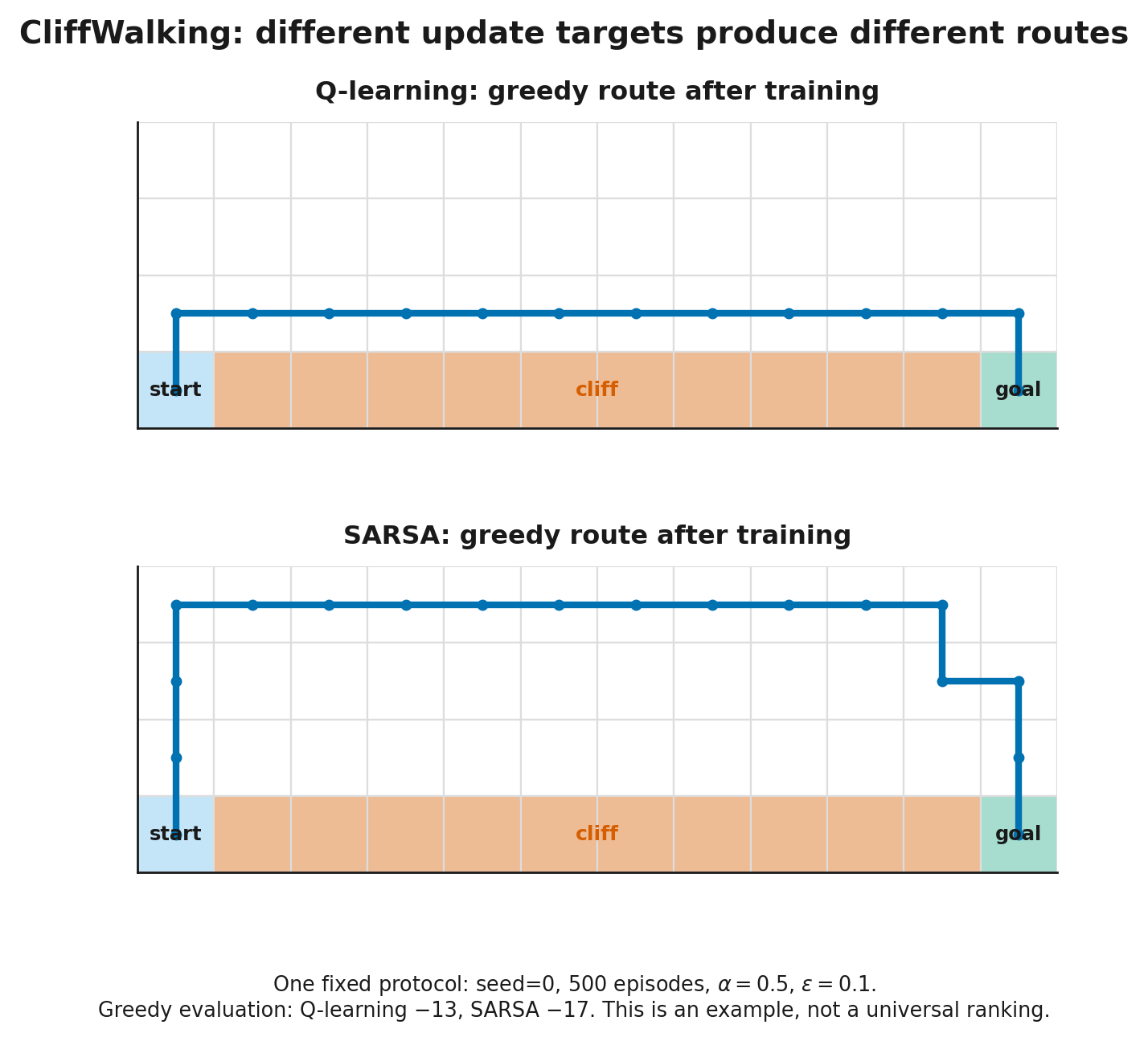
Reproduced results for this run are
| Method | Greedy-route return | Mean training return |
|---|---|---|
| Q-learning | ||
| SARSA |
Q-learning evaluates a greedy continuation and discovers the short route along the cliff. Actual exploratory behavior occasionally deviates and pays a large penalty. SARSA evaluates the continuation of that exploratory behavior and, in this run, learns a longer route with more margin.
This is not a universal ranking. Change , the penalty, episode budget, initialization, or evaluation rule and the numbers may move. The point is the causal relation between an update target and the risk represented in the learned function.
Step 2.4.4 — Why a maximum overestimates noisy values
Suppose several actions have equal true value but noisy estimates:
Each estimate may be unbiased on its own, yet the maximum selects the action that happened to receive a positive error:
This is maximization bias. Q-learning uses one table both to select the action and to evaluate it in the target, allowing selection noise to enter as an inflated continuation value.
Double Q-learning separates the two roles. When updating the first table, select with and evaluate with :
The tables can then swap roles. If their estimation errors are sufficiently independent, the positive error that drove selection in need not recur in . The method reduces typical overestimation, but it does not eliminate all error and can underestimate in some regimes.
There is a useful LLM analogy. When many responses are ranked by a noisy reward model and only the maximum is retained, the winner may benefit from evaluator noise as well as genuine quality. Separating generation, selection, and independent verification can reduce this effect. This is a shared statistical mechanism, not a claim that LLM reranking is literally Q-learning.
Step 2.4.5 — What transfers to LLM RL, and what remains a tabular teaching model
The module's durable ideas are:
- State is not merely an input record. It must be sufficient for future dynamics. A full prefix works for pure autoregression, while an external environment may make the task partially observable.
- , , and answer different questions. averages over the policy, fixes the first action, and compares an action with the current-policy average.
- A Bellman equation is one-step consistency, not a complete learning algorithm. It links present value to reward and continuation value.
- MC and TD choose where bootstrapping begins. MC observes the remaining return; TD substitutes a current estimate; multi-step targets connect the endpoints.
- Behavior and target policies may differ. That mismatch—not the mere presence of a replay buffer—makes Q-learning off-policy.
- Maximizing noisy estimates creates selection bias. Double Q-learning separates selection from evaluation and addresses one specific source of overestimation.
- The reason a trajectory stops belongs to the mathematics. True termination masks continuation; external truncation normally does not.
Tabular guarantees rely on finite spaces, a correct Markov model, sufficient exploration, and particular step-size schedules. LLM RL uses enormous spaces, neural approximators, potentially misspecified rewards, and a data distribution that moves with the policy. The equations provide a language and local training targets; they do not certify convergence of the complete system.
Abbreviation reference:
| Abbreviation | Full name | Role in this module |
|---|---|---|
| MDP | Markov decision process | fully observed Markov decision model |
| POMDP | partially observable Markov decision process | model with hidden environment state |
| MC | Monte Carlo | evaluation from observed returns |
| TD | temporal-difference learning | bootstrapped updating |
| GPI | generalized policy iteration | alternating evaluation and improvement |
| GAE | generalized advantage estimation | weighted combination of multi-horizon TD residuals |
| RMSE | root mean squared error | experiment error metric |
| EOS | end of sequence | sequence-termination token |
Sources and suggested reading path
Links were checked on August 4, 2026. Each item supports a specific part of the module and has an explicit boundary.
- Sutton & Barto, Reinforcement Learning: An Introduction, 2nd ed. — https://incompleteideas.net/book/the-book-2nd.html. The foundational source for finite MDPs, value functions, Bellman equations, MC, TD, SARSA, Q-learning, and GPI. Its tabular theory is not a proof of convergence for neural LLM training.
- Farama Foundation, “Handling Time Limits”. — https://gymnasium.farama.org/tutorials/gymnasium_basics/handling_time_limits/. Supports the practical
terminated/truncateddistinction and bootstrap rule. It is interface and environment-design guidance, not a universal theorem about every finite-horizon objective. - Watkins & Dayan, “Q-learning” (1992). — https://doi.org/10.1007/BF00992698. The primary source for classical tabular Q-learning and its convergence conditions. Those conditions should not be silently transferred to nonlinear approximation.
- van Hasselt, “Double Q-learning” (2010). — https://proceedings.neurips.cc/paper/3964-double-q-learning.pdf. The primary source for maximization bias and decoupled selection/evaluation. Double Q-learning reduces a characteristic overestimation mechanism; it is not universally unbiased.
- Schulman et al., “High-Dimensional Continuous Control Using Generalized Advantage Estimation”. — https://arxiv.org/abs/1506.02438. Connects multi-step temporal-difference residuals to GAE. Its policy-gradient role is deferred to Module 4.
- Shao et al., DeepSeekMath. — https://arxiv.org/abs/2402.03300. An author report describing the original GRPO group construction without a learned critic. It is not an independent replication of every empirical claim and does not cover all later variants.
- Official Gymnasium FrozenLake and CliffWalking pages. — https://gymnasium.farama.org/environments/toy_text/frozen_lake/ and https://gymnasium.farama.org/environments/toy_text/cliff_walking/. These document the canonical teaching environments. The numerical values in this course come from its own tested NumPy implementations under a stated protocol.
The expanded claim registry, verification status, and scope boundaries are in Module_2_Sources.md.
Next: Module 3, bandits and exploration. We temporarily remove multi-step dynamics and study the cost of exploration, upper-confidence methods, Thompson sampling, and the connection between choosing among several LLM responses and contextual bandits.