Module 3. Bandits, exploration, and one-step decisions
Material version: 2026.9
Factual snapshot: 2026-08-04
Language: EN
Core practice: browser, Python, and NumPy on a central processing unit (CPU); a separate English notebook joins bandit algorithms, logged-feedback evaluation, and LLM-style routing
Structure: 4 lessons, 21 steps
Estimated time: 7–10 hours, excluding the notebook’s full multi-run profile
Module 2 described the future consequences of an action through successor states and value functions. We will now remove the sequence for a while: the agent makes one decision, receives an immediate reward, and does not change the state of the next round. This is the bandit setting. It is simple enough for precise analysis, yet it isolates the central difficulty of exploration: how can an agent earn reward now while still collecting the information needed to make better decisions later?
No prior RL course is required. We will start from the definition, then introduce regret, upper confidence bound (UCB) methods and their classical UCB1 variant, Thompson sampling, and contextual bandits before transferring the ideas carefully to LLM systems. Readers who already know classical RL can move faster through the first two lessons and focus on logged-policy evaluation, the boundary of the bandit abstraction, the mathematics of Best-of-N, and the distinction between sampling temperature and exploration during learning.
Learning objectives. By the end of the module, you will be able to:
- distinguish stationary multi-armed and contextual bandits from a Markov decision process (MDP);
- compute expected regret and decompose it by the number of pulls of suboptimal actions;
- explain why pure greediness and constant random exploration can produce linear regret;
- implement ε-greedy, UCB1, and Thompson sampling for Bernoulli rewards;
- state the assumptions behind the logarithmic UCB1 guarantee and the scope of regret lower bounds;
- formulate a linear contextual bandit and interpret LinUCB, the linear UCB variant;
- evaluate a policy from logged feedback with inverse propensity scoring (IPS) and explain the overlap condition;
- explain when a complete LLM response can be treated as one action and when the bandit abstraction hides essential dynamics;
- derive the optimal one-step policy under entropy or Kullback–Leibler (KL) regularization;
- distinguish learning-time exploration, stochastic generation, Best-of-N, and pass@k;
- discuss entropy decline in reinforcement learning with verifiable rewards (RLVR) as an empirical failure mode rather than a universal law.
The learning platform places exercises after the relevant ideas and reveals a worked solution after an attempt or in the next step. The executable practice reproducibly compares exploration strategies, demonstrates non-stationarity, and builds the complete path from a logged interaction dataset to IPS, SNIPS, the direct method, and doubly robust evaluation. Verified claims and primary sources are registered in Module_3_Sources.md.
Practice route. Graded tasks, worked solutions revealed after an attempt, and executable practice follow the lecture. The explanation remains self-contained.
Lesson 3.1. One-step decisions and the price of uncertainty
Lesson 3.1. One-step decisions and the price of uncertainty
- What remains of RL when there is no next state
- The exploration–exploitation dilemma
- Cumulative reward, regret, and pseudo-regret
- Sample means and the greedy trap
- A reproducible testbed with more than one lesson
then 7 assessment steps
Step 3.1.1 — What remains of RL when there is no next state
In an MDP, an action affects both the immediate reward and the states the agent can reach later. A bandit removes that second link. On each round , the agent:
- chooses one of actions, ;
- receives a random reward ;
- observes only the reward of the selected action;
- proceeds to another independent round, without a controlled state transition.
In a stationary stochastic bandit, action has an unknown but fixed reward distribution with mean
The classical slot-machine metaphor calls actions arms. We will usually say “action” because the same equations can describe choosing a model, a request-processing route, or a response variant.
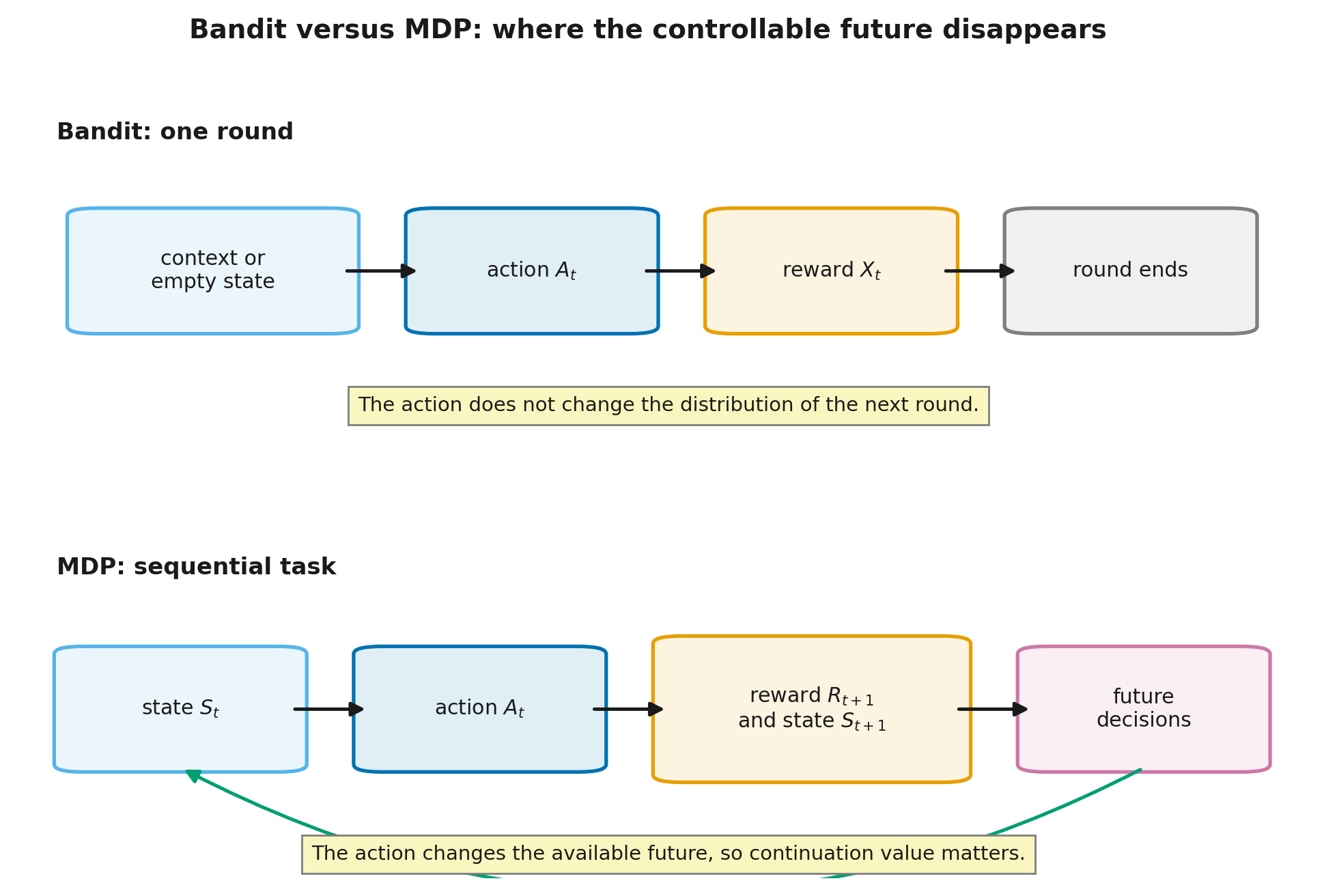
A bandit is not merely “RL without state notation.” It is a particular model with substantive assumptions:
- the action set is fixed;
- reward distributions are stationary;
- only the selected action's outcome is observed;
- an action does not change the context or reward distribution of the next round;
- rounds do not interfere with one another.
The last two points matter in practice. Rotating two headlines may be a bandit as long as showing one headline does not alter the future audience or its preferences. Managing a conversation, a robot, or a tool-using agent usually requires state because every action changes what happens next.
Practical test. If judging an action requires asking which state it will create and what will become possible afterward, the problem is no longer a pure bandit.
Step 3.1.2 — The exploration–exploitation dilemma
Let
be the mean reward of the best action. If all means were known, the agent would always choose an optimal action. They are not known, so the agent must solve two problems at once:
- exploit current knowledge by selecting the action with the largest estimate;
- explore alternatives that may be better than they currently appear.
Exploration has an immediate cost: the agent gives up the action that looks best. Refusing to explore has a delayed cost: an action that was lucky early on may be mistaken for the optimum forever.
The dilemma exists because the policy determines its own data. An action that is never selected produces no new evidence. A greedy policy can therefore maintain its own mistake: “I do not choose this action because I estimated it poorly; I estimated it poorly because I never choose it.”
The word exploration should not be stretched to cover all randomness. If an LLM with frozen weights samples several responses at high temperature, it produces diverse candidates, but its estimates and policy do not change. That is sampling or inference-time search. It becomes learning-time exploration only when feedback from those candidates affects later decisions.
Step 3.1.3 — Cumulative reward, regret, and pseudo-regret
One way to evaluate a strategy is its random cumulative reward,
For theory, it is convenient to compare its expectation with an oracle that knows the best action. The expected regret after rounds is
Under stationary rewards this equals expected pseudo-regret,
“Pseudo” does not mean unimportant. It means that random rewards have been replaced by their means. For a simulated trajectory whose true means are known, the realized quantity
contains no reward noise and is therefore convenient for reproducible comparisons.
Define the gap of action as
and its number of selections as
Then
That identity captures the entire mechanics of regret: every pull of a suboptimal action costs its gap . Most analyses therefore ask how often an algorithm returns to each suboptimal action.
- would mean a finite total price of uncertainty;
- means a slowly growing price;
- means that average loss vanishes;
- means a non-vanishing loss rate even at long horizons.
Not every problem admits logarithmic regret. The attainable rate depends on stationarity, the reward family, action separability, and the comparator used to define regret.
Step 3.1.4 — Sample means and the greedy trap
Suppose action has already been selected times and its current estimate is . After a new reward , the sample mean can be updated without storing the full history:
The pattern should look familiar from temporal-difference learning: old estimate plus step size times an error. Here there is no continuation value and no bootstrapping—the target is the observed one-step reward.
A purely greedy strategy chooses
If early noise makes a mediocre action look best, alternatives may never receive more data. Greediness finds the optimum quickly in some runs and becomes trapped in others; its average regret can therefore grow linearly.
Two elementary ways to break the loop are:
- ε-greedy: choose a random action with probability , otherwise act greedily;
- optimistic initialization: start with inflated values so that untested actions remain attractive.
A fixed never turns exploration off. When a suboptimal action exists, the random branch continues to choose it with positive frequency, so expected regret is usually linear. A decaying can achieve sublinear or logarithmic behavior, but only under an appropriate schedule and problem assumptions.
For non-stationary rewards, a sample mean may remember obsolete data for too long. A common alternative is a constant step size,
which exponentially downweights old observations. This is an engineering heuristic for tracking drift, not a free extension of stationary guarantees. The comparator changes as well: a non-stationary problem may call for dynamic regret against a changing optimum rather than regret against one fixed action.
Step 3.1.5 — A reproducible testbed with more than one lesson
Consider five Bernoulli actions with means
Protocol:
- horizon ;
- 400 independent runs;
- a separate fixed random stream for each algorithm;
- the plot shows mean pseudo-regret and a normal-approximation 95% confidence interval across runs;
- ties between greedy estimates are broken uniformly;
- UCB1 selects every action once before using its index;
- Thompson sampling uses priors.
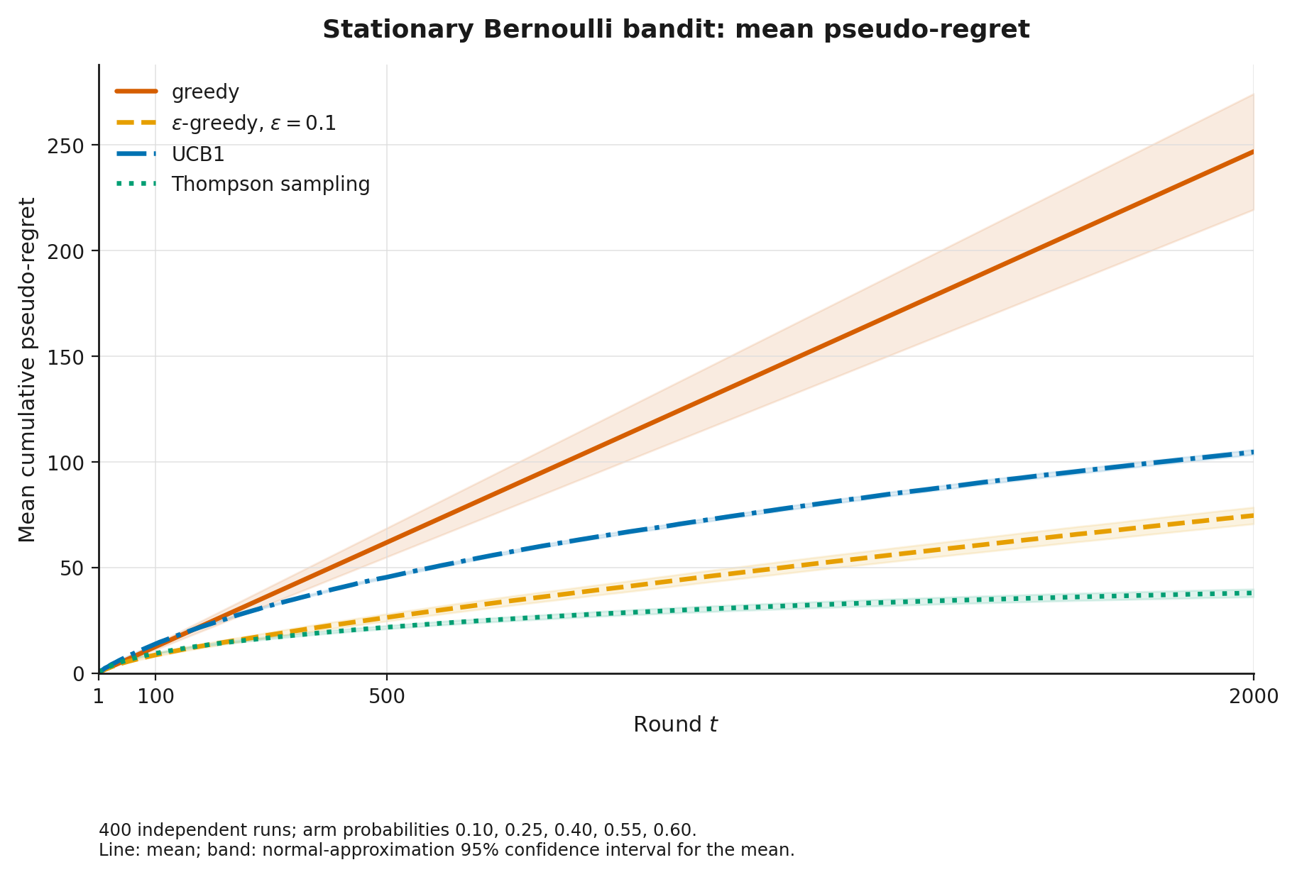
Mean pseudo-regret:
| Algorithm | Optimal-action rate at | |||
|---|---|---|---|---|
| Greedy | 12.54 | 61.84 | 246.72 | 0.297 |
| ε-greedy, | 8.64 | 26.34 | 74.55 | 0.684 |
| UCB1 | 13.88 | 45.39 | 104.60 | 0.586 |
| Thompson sampling | 9.37 | 21.72 | 37.92 | 0.786 |
The testbed is deliberately not presented as a universal ranking.
- Greediness gets trapped in a fraction of the runs.
- Constant ε helps but keeps paying for random actions.
- Canonical UCB1 explores conservatively here: with close means 0.55 and 0.60, its theoretical bonus remains noticeable for a long time.
- Thompson sampling has the lowest final regret in this protocol, but that is an empirical result for this instance, not an ordering that holds everywhere.
The numbers and plot are reproduced by module_3_reference.py and generate_m3_diagrams.py.
Lesson 3.2. Exploration directed by uncertainty
Lesson 3.2. Exploration directed by uncertainty
- From a confidence radius to a UCB index
- What UCB1 actually guarantees
- Thompson sampling
- UCB and Thompson sampling differ in more than randomness
- Stationarity, delayed feedback, and other boundaries
then 7 assessment steps
Step 3.2.1 — From a confidence radius to a UCB index
Uniform random exploration treats two very different cases alike:
- an action has been sampled three times and remains poorly understood;
- an action has been sampled three thousand times and is already estimated precisely.
An upper confidence bound (UCB) method adds an uncertainty bonus to the sample mean. For rewards in , Hoeffding's inequality gives
Choosing on the order of makes the event that the true mean lies above the constructed upper bound increasingly unlikely. The canonical UCB1 index is
Every action is selected once first, so the later index never divides by zero.
The first term exploits current estimates; the second explores uncertainty. The bonus:
- shrinks after new observations of that action;
- grows slowly when an action has been ignored;
- is largest where the estimate is least reliable.
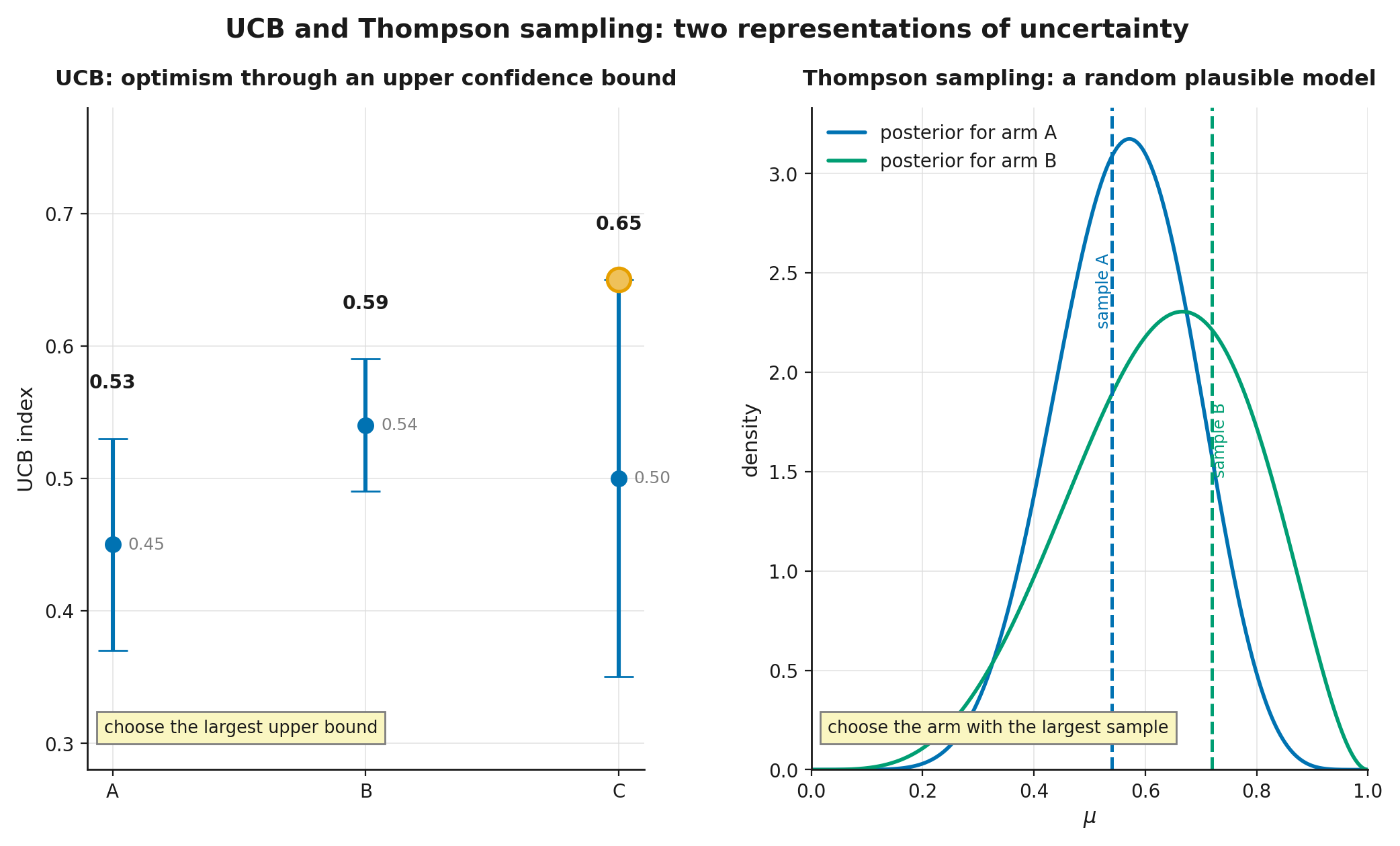
The phrase “confidence bound” refers to a mathematical object under stated assumptions. A neural system's arbitrary uncertainty score is not automatically a calibrated confidence bound.
Step 3.2.2 — What UCB1 actually guarantees
For stationary actions with independent rewards in and gaps , the UCB1 analysis gives, for every suboptimal action,
Multiplying by and summing yields
This is an instance-dependent bound. An action with a small gap is statistically difficult to distinguish from the optimum and may require many samples. Logarithmic asymptotics do not promise small regret at every finite horizon.
The Lai–Robbins lower bound also needs careful wording. For certain parametric reward families and uniformly efficient policies, a suboptimal action must asymptotically be sampled on the order of
where is Kullback–Leibler divergence between reward distributions. This does not imply that every algorithm on every conceivable instance must have regret exactly . Degenerate problems, extra structural information, or policies outside the uniformly efficient class can produce different rates. The conditions are part of the theorem, not fine print.
The practical conclusion remains: in the classical unknown stationary bandit, an algorithm cannot almost never inspect alternatives and still reliably rule them out.
Step 3.2.3 — Thompson sampling
UCB represents uncertainty with a deterministic bonus. Thompson sampling maintains a distribution over plausible parameters and acts according to one random hypothesis about the world on each round.
For Bernoulli rewards, the conjugate model is
After successes and failures, the posterior is
The algorithm then:
- samples from every current posterior;
- selects ;
- updates only the selected action's posterior.
Ignoring ties, an action is selected with the posterior probability that it is optimal. This is often called probability matching. A poorly observed action occasionally receives a high sample and is tested; its posterior narrows as evidence accumulates.
Thompson's original proposal dates to 1933 and concerned sequential allocation of observations. Modern regret guarantees and general theory came much later, so the historical date should not be treated as evidence for contemporary guarantees.
Step 3.2.4 — UCB and Thompson sampling differ in more than randomness
Both methods direct exploration using uncertainty, but they encode that uncertainty differently.
| Question | UCB | Thompson sampling |
|---|---|---|
| Representation of uncertainty | analytical upper index | posterior distribution over parameters |
| Action selection | usually a deterministic index maximum | maximum of random posterior samples |
| What must be specified | concentration assumptions and a bonus | probabilistic model and prior |
| Typical strength | transparent optimism-based guarantee | natural adaptive randomization |
| Typical failure mode | overly wide or miscalibrated bonus | misspecified likelihood or prior |
Neither column is an automatic recipe for an LLM system. An ensemble may provide a useful dispersion signal, but that dispersion need not be a Bayesian posterior. Token entropy is likewise not a confidence interval for the true utility of a response.
The robust transfer is more modest: exploration should respond to what the system does not yet know, rather than only to a fixed ε coin flip.
Step 3.2.5 — Stationarity, delayed feedback, and other boundaries
Classical formulas assume that an action's reward distribution is unchanged across rounds. Real systems violate this in several ways:
- the request population changes;
- users adapt to an interface variant;
- the base model is updated;
- rewards arrive with delay;
- the same user interacts repeatedly;
- an exposure changes the probability of future visits.
Drift can be addressed with sliding windows, discounting, or an explicit change model. Delayed rewards must not be silently recorded as zero before they arrive. Repeated interactions require a context that captures the relevant history—or a sequential model.
A tempting but invalid leap is: “UCB has logarithmic regret, so adding it solves any recommendation system.” The theorem applies to a particular statistical model. An engineering deployment must first justify that model and then separately validate calibration, delay handling, safety constraints, and the cost of exploration.
Lesson 3.3. Contextual bandits and logged feedback
Lesson 3.3. Contextual bandits and logged feedback
- One round, different situations
- Linear contextual bandits and LinUCB
- When an LLM response is one action
- Why a log does not contain every counterfactual
- Doubly robust evaluation and the limit of offline evidence
then 5 assessment steps
Step 3.3.1 — One round, different situations
A standard multi-armed bandit assigns one mean value to each action across all rounds. In many applications, however, the best action depends on the request, user, or task. A contextual bandit adds observed context :
- the environment reveals ;
- the policy chooses ;
- only is observed;
- the round ends.
The policy aims to maximize
for a deterministic policy, or the corresponding expectation over actions for a stochastic policy.
Context is not a state in the full MDP sense. It supports the current decision, but the chosen action is assumed not to change future context. If the response changes the conversation, user trust, or tool state, that assumption must be reconsidered.
Examples include:
- context: user features; action: recommendation; reward: click;
- context: clinical features; action: treatment; reward: observed outcome;
- context: request; action: one of several models; reward: quality adjusted for latency and cost;
- context: prompt; action: complete response; reward: a scalar score, after which the episode ends.
The last example connects bandits to LLM alignment without claiming that internal token generation has stopped being sequential.
Step 3.3.2 — Linear contextual bandits and LinUCB
Let every context–action pair have a feature vector
and suppose expected reward is approximately linear:
After observations , ridge regression gives
LinUCB selects an action using
The first term is predicted reward; the second is an elliptical bonus for a feature direction poorly covered by past data. Two actions may have the same pull count yet different uncertainty because their feature vectors occupy differently explored directions.
LinUCB is a transparent mechanism, but linearity is a substantive assumption. Feeding an LLM embedding into a linear head does not prove that true reward is linear in that embedding or that the bonus is calibrated. A real system still needs held-out and controlled online validation.
Step 3.3.3 — When an LLM response is one action
For a single request, define:
- context as the prompt and available metadata;
- action as a complete response;
- reward as a human score, reward-model output, or verifier result;
- termination immediately after the score is produced.
Under this whole-response external abstraction, the problem is indeed a contextual bandit. InstructGPT, for example, explicitly describes its environment as a bandit that presents a prompt, receives one response, returns a scalar reward, and ends the episode.
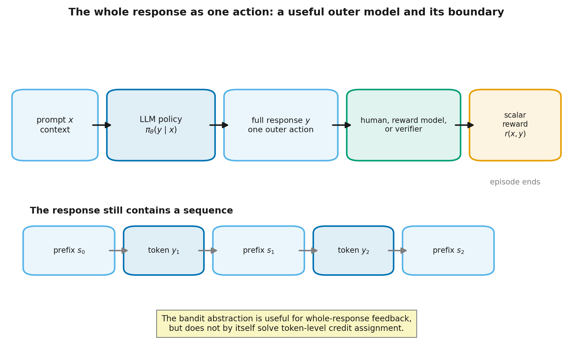
Inside the action , however, autoregressive factorization remains
Both views are therefore valid at once:
- externally, the complete response is one contextual-bandit action;
- internally, tokens are sequential actions and the prefix is state.
The right abstraction depends on the question. A bandit is useful for comparing finished responses. It hides essential structure for token-level credit assignment, length control, tool use, and multi-turn interaction.
Boundary of the transfer. “Single-turn alignment can be represented as a contextual bandit” is exact under a whole-response reward and terminal round. “All LLM training is a bandit” is not.
Cross-reference: data preparation and supervised fine-tuning (SFT) are covered in Modern LLMs, Module 13 “Supervised Fine-Tuning and Data Work” (modern_llms.module_11_sft), while the architecture-level map of RLHF, DPO, and GRPO is in Module 14 “Learning from Feedback: RLHF, DPO, RLOO, and GRPO” (modern_llms.module_12_preference_optimization). This module remains the canonical treatment of one-step feedback statistics.
Step 3.3.4 — Why a log does not contain every counterfactual
A deployed system often records tuples
where is the probability with which the behavior policy selected the displayed action. Rewards for unchosen actions are missing.
To evaluate a new policy without immediate deployment, inverse propensity scoring (IPS) uses
The weighting identity, conditional on and potential rewards, is
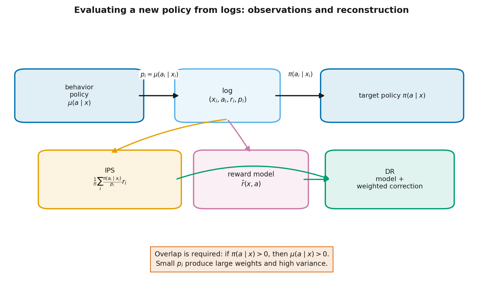
Unbiasedness needs important conditions:
- overlap: if , then ;
- stored propensities match the actual randomized choice mechanism;
- reward and context are logged correctly;
- conditional on the recorded context, the action does not depend on an unrecorded factor that also affects the potential reward; correct randomization or a defensible assignment model is needed.
Small values create large weights and high variance. The self-normalized inverse propensity scoring (SNIPS) estimator is
This estimator is often numerically more stable, but it is generally biased.
This is why production logging should retain action probabilities, policy versions, randomization details, and timestamps. Without them, historical data may be unusable for a defensible policy evaluation.
Step 3.3.5 — Doubly robust evaluation and the limit of offline evidence
IPS uses a behavior-policy model but may have large variance. A direct reward model avoids extreme weights but can be biased by misspecification. A doubly robust (DR) estimator combines both:
The first term predicts the new policy's reward. The second corrects that prediction on actions that were actually observed. Under standard conditions, the estimate remains consistent if at least one of the two models is correct: the reward model or the behavior propensity model. “Doubly robust” refers to that structure.
DR still cannot create evidence where overlap is absent. If the new policy selects an action that the old policy never displayed in a context, the counterfactual reward is not identified by the logs alone. A model can extrapolate, but that is an extra assumption rather than a consequence of the data.
The issue is acute for LLMs: complete-response spaces are enormous, exact string probabilities may be tiny, and semantically similar responses are still distinct actions. Whole-response IPS is therefore often impractical. More realistic applications restrict the action set, evaluate routing among models or templates, impose structure on the policy, or run a controlled online experiment.
Lesson 3.4. Entropy, temperature, and multiple candidates
Lesson 3.4. Entropy, temperature, and multiple candidates
- Entropy-regularized one-step decisions
- Sampling temperature is not learning-time exploration
- Best-of-N: an exact probability and an imprecise “bandit” label
- pass@k: population probability versus a finite-sample estimate
- Entropy decline in RLVR: an observed regime, not a theorem
- Final map and the bridge to policy gradients
then 7 assessment steps
Step 3.4.1 — Entropy-regularized one-step decisions
Suppose a finite set of actions has known quality scores . Maximizing only expected quality,
places all probability on a maximizing action. Add entropy
with coefficient :
The Lagrangian for gives
and therefore
Temperature controls the trade-off between quality and entropy: as , the policy concentrates on a maximum; at high , it approaches uniformity.
A more general formulation penalizes the Kullback–Leibler (KL) divergence from a reference policy :
has solution
This is an exact one-step result. It does not claim that arbitrary neural optimization reaches the distribution or that the score is correct.
Mathematical deepening: Information Theory for ML, Module 8 “Maximum entropy, exponential models, and KL regularization” (it_ml.module_08_maxent_kl_policy) derives the variational result, Gibbs form, and normalizing constant in detail. The present module is still self-contained: the equations and their interpretation have been derived here.
Step 3.4.2 — Sampling temperature is not learning-time exploration
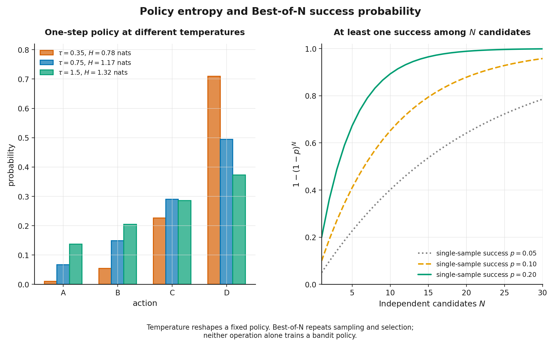
For fixed logits , decoding temperature defines
Raising flattens a pure softmax distribution and increases its entropy; lowering it concentrates probability. Three boundaries matter:
- the statement assumes fixed logits, whereas training changes the logits themselves;
- temperature changes the candidate distribution but does not update quality estimates;
- after top-, top-, token bans, and other filters, the final distribution is not described by one pure temperature curve. A token assigned zero probability by a filter cannot be restored by temperature alone.
It is therefore useful to separate:
- learning-time exploration: actions produce feedback that changes the future policy;
- stochastic generation: a fixed policy produces different candidates;
- inference-time search: the system spends additional compute selecting, checking, or improving candidates.
The mechanisms may be combined, but they are not synonyms. Decoding, candidate selection, and inference-time computation are treated more broadly in Modern LLMs, Module 15 “Reasoning Models and Test-Time Compute” (modern_llms.module_13_reasoning).
Step 3.4.3 — Best-of-N: an exact probability and an imprecise “bandit” label
Assume each independent candidate succeeds with probability , and an ideal verifier selects a successful candidate whenever one exists. The probability of at least one success among candidates is
For ,
and reaching at least 90% requires
so the minimum is 11 independent candidates.
The mathematics is exact under strong assumptions:
- candidates are independent and identically distributed;
- the verifier identifies success without error;
- generation and verification cost is absent from the objective;
- the selected response does not affect future tasks.
Ordinary Best-of-N from a fixed LLM is not a standard finite-armed online bandit. There is no fixed set of unknown arms whose values are estimated over repeated rounds. It is repeated sampling from one policy followed by selection with a verifier or ranker.
A true bandit appears when a system repeatedly chooses among models, prompts, temperatures, or processing routes and updates those choices from feedback. The presence of several candidates alone is not enough.
A real ranker can also make mistakes. Then selected-response quality depends both on whether a good candidate exists and on whether the ranker recognizes it. The formula is the ideal-verifier ceiling in the stated model, not a guarantee of deployed quality.
Step 3.4.4 — pass@k: population probability versus a finite-sample estimate
In code generation, pass@ asks for the probability that at least one of candidates passes the tests. If one independent candidate succeeds with true probability , then
In an evaluation, however, is unknown. Suppose programs are sampled for one task and of them pass. Plugging into gives a biased estimator. The Codex evaluation uses the following finite-sample estimator:
This is the probability that a uniformly selected size- subset without replacement contains at least one of the successful programs. Estimates are then averaged over tasks.
Keep the two quantities distinct:
- is a population formula for independent, identically distributed samples;
- the combinatorial expression estimates pass@ from a finite set already generated.
Near-duplicate candidates provide less effective diversity than an independence intuition suggests. Higher temperature may sometimes improve diversity while reducing single-sample quality; the best operating point depends on the model, task, and budget. Module 13 of this course, “Evaluation, Reward Hacking, and Safety” (rl_llm.module_13_evaluation), returns to the broader evaluation protocol.
Step 3.4.5 — Entropy decline in RLVR: an observed regime, not a theorem
In reinforcement learning with verifiable rewards (RLVR), a model receives an automatically checkable signal, such as mathematical correctness or passing program tests. One discussed failure mode is entropy collapse: token distributions become overly concentrated too early, trajectory diversity falls, and optimization may stall.
For state , token entropy is
A decline in average is not inherently wrong: a successful policy often should become more decisive. The concern is premature loss of diversity before the solution space has been explored, or concentration caused by optimization pathology rather than durable reward improvement.
A 2026 preprint reports substantial entropy decline in several RLVR configurations on mathematical reasoning tasks and analyzes how updates to individual tokens contribute to entropy change. That is a primary empirical report from one study, not proof that every run of group relative policy optimization (GRPO) must collapse.
A small piece of algebra explains one source of missing signal in GRPO. If all responses for one prompt receive the same reward,
then mean centering gives
for every response. Under the standard group normalization, relative advantages are zero if other objective terms are ignored. The group supplies no preference over its samples. This is not a complete theory of entropy dynamics, but it is an exact local boundary: without variation in feedback, the relative group signal vanishes.
Module 9 of this course, “RLVR and GRPO: Verifiable Reward, Group-Relative Estimation, and Stability” (rl_llm.module_09_rlvr_grpo), returns to GRPO, clipping, policy ratios, group construction, and RLVR through the full objective.
Step 3.4.6 — Final map and the bridge to policy gradients
The module separated several mechanisms that can look superficially similar.
| Mechanism | What is unknown | What changes after feedback | Main risk |
|---|---|---|---|
| Stationary bandit | action reward means | estimates and later action choices | too little or too much exploration |
| Contextual bandit | reward as a function of context and action | policy for future contexts | missing overlap, misspecification |
| Temperature sampling | no estimate is updated | only the current candidate set | confusing diversity with learning |
| Best-of-N | candidate success probability and verifier error | usually nothing in model weights | correlated candidates, ranker error |
| Entropy regularization | quality–entropy trade-off | optimized policy | misspecified reward or excess regularization |
| RLVR | trajectory quality under a verifier | LLM parameters | low diversity, sparse signal, verifier exploitation |
The main conclusions are:
- a bandit is a precise one-step model, not a generic word for choice;
- regret measures the price of uncertainty against an explicit comparator;
- UCB and Thompson sampling direct exploration through uncertainty but represent it differently;
- a contextual bandit is useful for the one-step abstraction that rewards a complete LLM response, but it does not replace token-level MDPs or multi-turn environments;
- offline evaluation requires behavior propensities and overlap;
- temperature, Best-of-N, and pass@ concern generation and evaluation, not automatically learning-time exploration;
- entropy is a property of an action distribution, not a measure of answer truth.
Module 4 of this course, “Policy Gradients: from REINFORCE to PPO” (rl_llm.module_04_policy_gradients), restores sequential decision making and changes the parameters of a stochastic policy directly. The bandit will become the simplest policy-gradient case: an action is already sampled from ; the remaining question is how its reward yields an unbiased gradient of expected performance.
Acronym reference
| Acronym | Full form | Role in this module |
|---|---|---|
| MDP | Markov decision process | sequential model contrasted with a bandit |
| UCB | upper confidence bound | estimate plus uncertainty bonus |
| IPS | inverse propensity scoring | target-policy evaluation from logged actions |
| SNIPS | self-normalized inverse propensity scoring | self-normalized IPS variant |
| DR | doubly robust | estimator combining reward prediction and propensity weights |
| RLVR | reinforcement learning with verifiable rewards | training from automatically checkable reward |
| GRPO | group relative policy optimization | family of group-relative policy updates |
| KL | Kullback–Leibler | divergence from a reference distribution |
Completion check: you should be able to explain why Best-of-N is not automatically a multi-armed bandit, derive the regret decomposition by , interpret a UCB bonus, update a Beta posterior, state the overlap condition for IPS, and separate sampling temperature from learning-time exploration.
Practical route
- a multi-run comparison of ε-greedy, UCB1, and Thompson sampling;
- adaptation after the best arm changes in a non-stationary environment;
- a contextual-bandit log with a known behavior policy;
- IPS, SNIPS, the direct method, and doubly robust evaluation;
- an overlap stress test with weight concentration and effective sample size;
- LLM-style model routing with explicit quality, cost, and latency terms.
The learning platform adds 32 exercises with worked solutions revealed after an attempt. The default profile runs on CPU; the full profile increases the number of repeated runs for more stable curves, but it does not turn the course experiment into an external benchmark.
Sources and a route for further reading
- Lattimore and Szepesvári, Bandit Algorithms — a systematic treatment of stochastic and contextual bandits, regret, and lower bounds. Its theorems apply to explicit bandit classes, not automatically to arbitrary neural uncertainty scores.
- Auer, Cesa-Bianchi, and Fischer, “Finite-time Analysis of the Multiarmed Bandit Problem” — the primary finite-time UCB1 result for bounded rewards. It does not license every “estimate plus bonus” heuristic.
- Thompson, “On the Likelihood that One Unknown Probability Exceeds Another…” — the historical source of probability matching. Modern Thompson-sampling guarantees require later analysis.
- Li et al., “A Contextual-Bandit Approach to Personalized News Article Recommendation” — LinUCB and a concrete contextual setting. Linear reward structure remains an assumption, not a property conferred by arbitrary embeddings.
- Ouyang et al., “Training Language Models to Follow Instructions with Human Feedback” — an example of treating a complete response as one external bandit action during InstructGPT PPO training. Internally, generation remains token-sequential.
- Dudík, Langford, and Li, “Doubly Robust Policy Evaluation and Learning” — the primary doubly robust evaluation source. Double robustness does not repair absent overlap, hidden confounding, or corrupted behavior probabilities.
- Chen et al., “Evaluating Large Language Models Trained on Code” — the source of the finite-sample pass@ estimator. It is not the same object as the population formula .
- Xu et al., “Understanding and Preventing Entropy Collapse in RLVR with On-Policy Entropy Flow Optimization” — a 2026 primary report of entropy decline in the authors’ studied RLVR settings. The module treats it as a contemporary observation, not a universal theorem.
Module_3_Sources.md contains the full claim registry, evidence classes, and scope limits.