Module 4. Policy gradients: from REINFORCE to PPO
Material version: 2026.9
Factual snapshot: 2026-08-04
Language: EN
Core practice: browser, Python, and NumPy on a central processing unit (CPU); a separate English notebook joins REINFORCE, GAE, a complete CartPole PPO implementation, and an autoregressive LLM-style example
Structure: 5 lessons, 25 steps
Estimated time: 9–13 hours, excluding the notebook’s full multi-seed profile
Module 2 improved behavior through value functions, while Module 3 studied one-step decisions. We now take a different route: optimize the policy parameters directly. This route is central for LLMs because the final reward may come from a person, an executable verifier, or a non-differentiable scoring model. No gradient passes through that feedback directly.
No previous RL course is required. We begin with a gradient estimator for parameterized distributions, then build REINFORCE, baselines, actor–critic methods, generalized advantage estimation, and proximal policy optimization (PPO). Readers with a classical RL background can treat the first two lessons as a precise refresher and focus on finite-group bias, correct time-limit handling, and trajectory versus local probability ratios. Group-based estimators for several responses appear only after the common foundation is in place.
Module goals. After completing the module, you will be able to:
- derive the log-derivative identity and the REINFORCE estimator;
- explain when environment dynamics disappear from the derivative but remain in the data distribution;
- distinguish the gradient of the literal discounted objective from the common discounted-occupancy convention;
- prove why an action-independent baseline leaves the expected policy gradient unchanged;
- distinguish the natural baseline from the exact variance-minimizing scalar baseline;
- compute same-group and leave-one-out advantages;
- implement generalized advantage estimation (GAE) with separate masks for termination and time-limit truncation;
- derive the local surrogate and clipped PPO objectives;
- read core PPO diagnostics without mistaking them for universal guarantees;
- connect sequence-level REINFORCE to an estimator that leaves the current response out of its baseline, and distinguish that construction from the broader family of group-based methods.
The learning platform places exercises after the relevant ideas and reveals a worked solution after an attempt or in the following step. The executable practice implements the complete path from rollouts and GAE through repeated PPO epochs, then carries the same mechanics into an autoregressive-response example. Verified claims and primary sources are recorded in Module_4_Sources.md.
Practice route. Graded tasks, worked solutions revealed after an attempt, and executable practice follow the lecture. The explanation remains self-contained.
Lesson 4.1. Estimating a policy gradient and REINFORCE
Lesson 4.1. Estimating a policy gradient and REINFORCE
- Optimizing the policy directly
- The log-derivative identity
- Trajectory probability and the disappearance of the environment model
- Causality and reward-to-go
- The policy-gradient theorem and REINFORCE
then 6 assessment steps
Step 4.1.1 — Optimizing the policy directly
Let a parameterized policy generate trajectories, and let the objective be expected return:
In ordinary supervised learning, the data are fixed and the derivative flows through the loss. In RL, the data distribution itself depends on : changing the policy changes actions, states, and future observations. The operation “sample an action” is also discrete. We therefore cannot simply backpropagate through a selected token or through an external verifier.
That does not make the objective gradient unavailable. We need an estimator that:
- uses samples from the current policy;
- does not differentiate the reward;
- does not differentiate the sampling operation;
- remains valid for discrete actions.
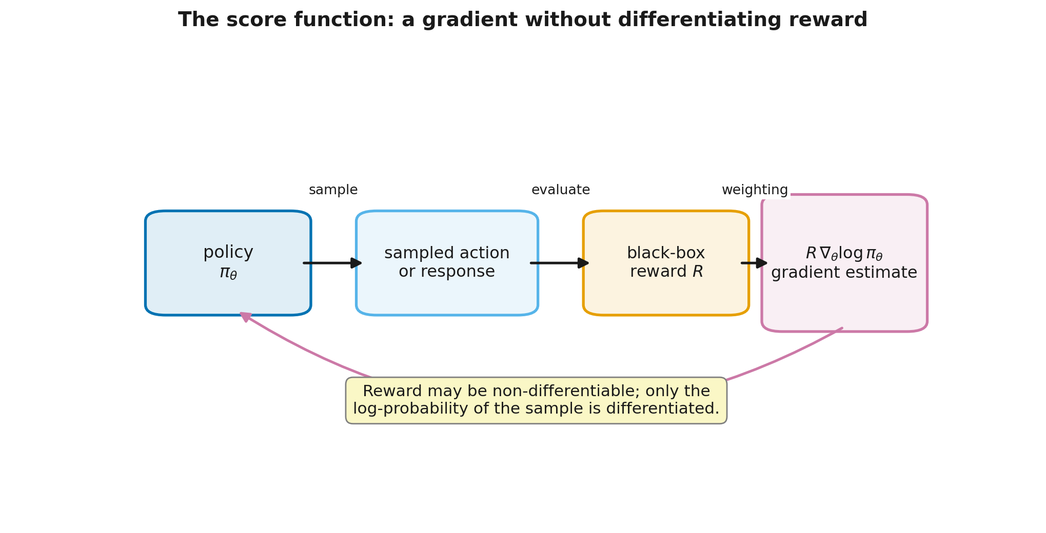
The log-derivative identity provides exactly this construction. The resulting multiplier is called the score function. Here, “score” is a statistical term: it is the derivative of a log-density or log-probability with respect to model parameters, not the reward value.
For an LLM, the picture is simple: the model samples a token sequence, a verifier returns a number, and the optimizer must infer how to change the probabilities of the sampled tokens. The next steps turn that picture into an equation.
Step 4.1.2 — The log-derivative identity
For a discrete random variable and a function with no direct dependence on ,
Use
Then
The expectation can be estimated from independent samples:
This is the central trade: we avoid differentiating , but pay Monte Carlo variance. The construction still works when is a compiler result, a human rating, or a binary verifier output.
The phrase “no direct dependence on ” is not decorative. If the integrand is , the product rule produces two terms:
The first term accounts for the changing distribution of outcomes; the second accounts for the integrand changing at a fixed outcome. Classical REINFORCE treats environment reward as fixed with respect to policy parameters, so the direct term vanishes. A differentiable regularizer built from the current policy is different: an implementation must either retain its direct derivative or deliberately stop that gradient and thereby define a different computational objective.
As usual, differentiation and summation or integration must be interchangeable. This is typically straightforward in a finite action space; continuous spaces require the relevant regularity conditions.
For a softmax policy with logits ,
where is the one-hot vector of the sampled action. A positive coefficient raises that action's logit relative to the others; a negative coefficient lowers it.
Step 4.1.3 — Trajectory probability and the disappearance of the environment model
Consider a finite trajectory
If the initial distribution and environment dynamics do not depend on , its probability factorizes as
The logarithm turns the product into a sum. Differentiation with respect to acts only on the policy:
Substituting into the score-function identity gives
The phrase “the environment dynamics disappear” needs a precise reading. They disappear from the explicit derivative, but still determine which trajectories are observed and which rewards the agent receives. If transitions share parameters with the policy, if the environment is trained jointly, or if we explicitly differentiate through a known simulator, the simplification no longer captures the full derivative.
For LLM training, an external verifier normally does not depend on policy weights, so its derivative is unnecessary. Yet it still defines the training signal: a flawed verifier gives a valid gradient of the wrong objective.
Step 4.1.4 — Causality and reward-to-go
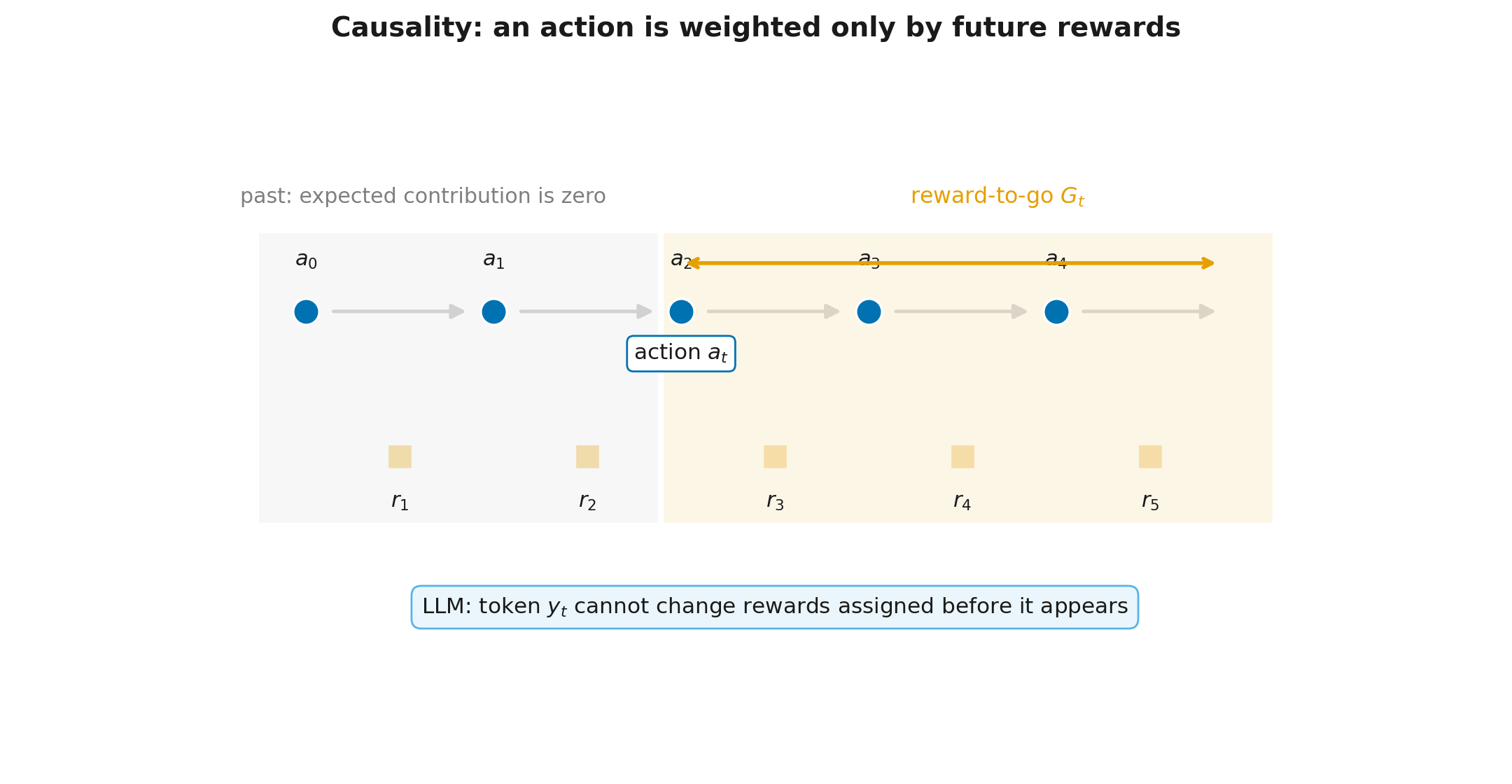
In the previous equation, every score term was multiplied by the full trajectory return. Action , however, cannot affect rewards received before time . Their expected contribution vanishes because the conditional mean of the score is zero:
The full return can therefore be replaced by reward-to-go:
For the literal objective
a direct derivation yields the weight :
Textbooks often display the equation without the outer . That form generally adopts a different convention: discounting has already been absorbed into the state-occupancy measure, or the objective weights decision times differently. Dropping the factor is not always a harmless global rescaling. In a finite-horizon problem it changes the relative weight of early and late decisions and can therefore change the gradient direction. An implementation may deliberately choose that objective for optimization reasons, but the derivation, code, and interpretation must use the same convention.
Step 4.1.5 — The policy-gradient theorem and REINFORCE
Using a discounted occupancy measure, the policy-gradient theorem can be written as
The proportionality constant depends on how the occupancy measure is normalized. The practical interpretation is stable: raise an action's probability when its expected continuation is above the reference level, and lower it when it is below.
REINFORCE, introduced by Ronald Williams, replaces the unknown with a sampled return:
- collect trajectories with the current policy;
- compute or the chosen discounted score weight;
- form
- take a gradient-ascent step.
Under correct sampling, the estimator is unbiased for the chosen objective, but it may have high variance. “Unbiased” does not mean “learns quickly”: a single batch can point in an almost arbitrary direction. The next lesson develops control variates that reduce noise without changing the expected gradient.
For an LLM, the log-probability of a trajectory becomes the sum of token log-probabilities. We keep the reward at whole-response level for now and return to token-level credit in Lesson 4.5.
Lesson 4.2. Baselines and group estimators
Lesson 4.2. Baselines and group estimators
- What can be subtracted without changing the expectation
- Why the state value is natural but not always variance-minimizing
- The same-group mean and dependence on the current sample
- Leaving the current response out of the baseline
- A reproducible experiment on expectation and variance
then 4 assessment steps
Step 4.2.1 — What can be subtracted without changing the expectation
Let be any state-dependent function that does not depend on the sampled action. Then
Consequently,
without changing the expected gradient. This construction is a control variate, and is a baseline.
Choosing
turns the coefficient into the advantage
A positive coefficient now means not merely “the return was positive,” but “the action did better than the usual continuation from this state.” This removes the pointless tendency to reinforce every action in a task where all episodes carry a large positive constant.
Action independence is essential. Subtracting an arbitrary generally changes the expectation. More elaborate action-dependent control variates exist, but they require correction terms and are outside the core route.
Step 4.2.2 — Why the state value is natural but not always variance-minimizing
is a natural baseline: it turns into an advantage and fits the actor–critic architecture. But “ always minimizes policy-gradient variance” is too strong.
At a fixed state, consider a scalar baseline and the vector estimator
Minimizing its second moment with respect to gives
The state value
matches only when the squared score norm is uncorrelated with or nearly constant across actions. In a neural network, the exact optimum also depends on which parameter coordinates and norm define variance.
This qualification does not make a poor choice. It is easy to learn by regression, has a clear interpretation, and often reduces variance substantially. It is an effective approximation, not a universal exact minimizer.
The analytical exercise gives a sharp example: with logits and action values , while .
Step 4.2.3 — The same-group mean and dependence on the current sample
For an LLM prompt, it is often possible to generate several responses. Let conditionally independent responses have rewards and scores .
The simplest baseline is the mean of the same group:
The advantages sum to zero, but includes itself. It is therefore not independent of the current sampled action. Under conditional independence, the expectation is
The expected direction is preserved, but the magnitude is scaled by . A fixed group size lets the optimizer absorb this factor into the learning rate, yet the estimator should not be called literally unbiased.
Dividing centered rewards by the sample standard deviation introduces another random normalization. This can stabilize update scale, but it is no longer a simple expectation-preserving control variate. If all rewards are equal, the standard deviation vanishes and practical code returns zero advantages with an safeguard.
Step 4.2.4 — Leaving the current response out of the baseline
Remove the current response from the group mean:
For conditionally independent responses, does not depend on , so the estimator retains the correct expectation. Within one group,
Same-group centering and leave-one-out centering therefore produce collinear coefficients, but with different finite-sample scale.
REINFORCE leave-one-out (RLOO) applies this idea to several responses for one prompt. In its simplest whole-response form, each reward is compared with the mean reward of the other responses, and the resulting advantage multiplies the sum of token log-probabilities.
The assumptions matter:
- responses should be sampled from one frozen policy;
- cross-response reward noise should not create complex dependence on the current response;
- token aggregation and masks must be specified for variable-length responses;
- RLOO still provides no token-level explanation of which part of a response earned the reward.
Step 4.2.5 — A reproducible experiment on expectation and variance
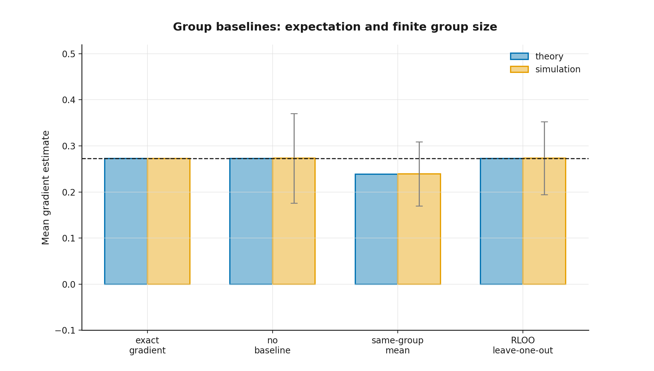
Consider a one-step Bernoulli policy
with . The reward is for and for . The exact gradient with respect to the logit is
For group size , the same-group mean estimator has predicted expectation
module_4_reference.py generates independent groups and compares:
- no baseline;
- the in-sample group mean;
- leave-one-out centering.
The simulation confirms the expected means. It does not establish a universal variance ranking: variance depends on the policy, reward distribution, group size, and parameterization. The purpose is to separate two questions that are often conflated: whether an estimator has the right expectation and how noisy it is in a specific setting.
Lesson 4.3. Actor–critic methods and generalized advantage estimation
Lesson 4.3. Actor–critic methods and generalized advantage estimation
- The critic as a learned baseline
- Temporal-difference residuals and multi-step targets
- Generalized advantage estimation
- Termination, time-limit truncation, and rollout boundaries
- A complete actor–critic cycle
then 3 assessment steps
Step 4.3.1 — The critic as a learned baseline
In a large state space, we cannot repeatedly revisit each state and average future returns. Instead, we learn
where parameterizes the critic and parameterizes the actor, the policy. This gives an actor–critic architecture:
- the actor selects actions and receives a policy-gradient update;
- the critic predicts expected continuation return;
- the difference between a target and the critic prediction estimates advantage.
The critic need not be a separate network. In LLM systems, a shared transformer may carry an additional value head. The logical roles remain distinct: the policy defines an action distribution, while the critic predicts expected return.
A common critic loss is
A noisy or biased target gives the critic the same defects. A poor critic can increase rather than decrease actor-update variance. Value loss, explained variance, and advantage scale are therefore substantive diagnostics, not bookkeeping.
The computational graph has an equally important contract. During the actor update, is normally treated as an already computed numerical coefficient: gradients through the critic and through target construction are stopped (detach / stop-gradient). Otherwise the actor loss can inadvertently train the critic or alter the advantage estimator itself. The critic receives its own gradient from . This does not forbid a shared backbone: if actor and critic share representations, the combined loss may still update shared parameters, but each branch must have an explicit gradient route.
Step 4.3.2 — Temporal-difference residuals and multi-step targets
The one-step temporal-difference (TD) residual is
If , its conditional expectation given equals . With an approximate critic, it is biased but local and often lower-variance.
Looking farther ahead gives
At this is a TD estimate; extending to the end of the episode gives a Monte Carlo return minus the value. Increasing reduces dependence on critic error but adds randomness from future rewards and actions.
There is no universal rule that longer targets are better. In a deterministic environment, a long target may be nearly noiseless. In a stochastic dialogue or tool-use task, it can have enormous variance. We need a controlled mixture of horizons.
Step 4.3.3 — Generalized advantage estimation
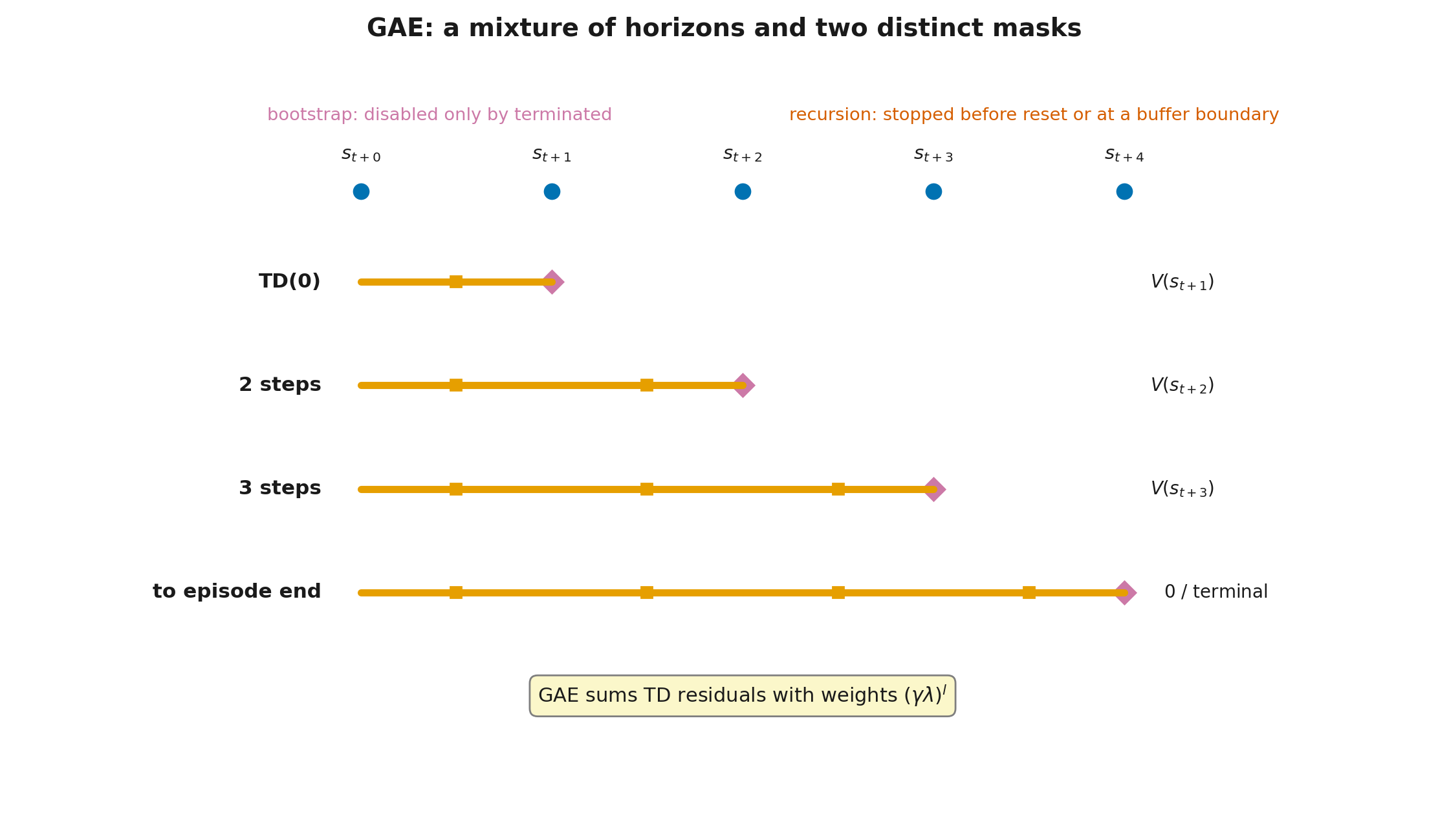
Generalized advantage estimation (GAE) mixes multi-step estimates with geometric weights. Its convenient backward recursion is
Equivalently,
where is the available uninterrupted suffix before a true terminal, an environment reset, or a computational rollout boundary. The parameter selects the mixture:
- leaves the one-step TD residual;
- intermediate values combine several horizons;
- at , the residual sum does not merely resemble a long target—it telescopes.
If the uninterrupted fragment ends at index and its final next state uses the correct value , then
At a true terminal, the final value is zero and the expression becomes Monte Carlo return minus . At the boundary of a collected rollout, the environment may continue, so the bootstrapped tail remains. Short buffers and long conversations make this distinction operational rather than cosmetic.
After advantages are computed, a common critic target is
The old prediction, the advantage estimate, and the regression target are three different objects. Normalizing advantages for the policy update should not silently normalize the critic target as well.
Step 4.3.4 — Termination, time-limit truncation, and rollout boundaries
A codebase may expose one convenient done flag, but the mathematics benefits from separating at least three cases.
- True termination. The task has reached a terminal state; the specified process has no continuation.
- Time-limit or external truncation. The environment is reset because an external limit was reached even though the final state may have nonzero continuation value.
- A rollout-buffer boundary. The collector stops the current fragment after a fixed number of transitions, while the environment neither terminates nor resets. The next fragment may continue the same episode.
Value bootstrap is controlled by whether a true continuation exists:
The backward recursion answers a different question: is available inside the fragment currently being processed?
trace_cut is one before an environment reset and at the end of a local buffer when the next advantage is not present in that array. At a time-limit truncation, bootstrap from the final observation before reset(), but do not recurse into the first state of the next episode. At an ordinary rollout boundary, bootstrap from the next observation as well; a streaming implementation may carry recursion state into the next fragment, whereas a batch implementation stops locally and represents the tail through .
| Event | Bootstrap from next state | Recurse inside the current array |
|---|---|---|
| True termination | no | no |
External truncation followed by reset() | yes, from the final observation | no |
Buffer boundary without reset() | yes | no, unless fragments are joined |
| Ordinary transition | yes | yes |
A common bug uses one done flag to disable both bootstrap and recursion. That conflates two independent questions and biases targets near time limits. Removing a positive continuation value lowers the target; removing a negative one raises it, because the omitted term is . For example, with zero reward, , and , the target incorrectly changes from to . In LLM rollouts, the analogous distinction is among a naturally sampled end-of-sequence token (EOS), a forced max_tokens cutoff, and an infrastructure boundary that merely closes the current rollout batch.
Step 4.3.5 — A complete actor–critic cycle
One on-policy actor–critic iteration is:
- freeze the current policy ;
- collect trajectories and store actions, old log-probabilities, rewards, value predictions, and masks;
- compute and value targets ;
- update the actor with a policy-gradient estimate;
- update the critic by regression to ;
- collect fresh data after the policy has changed enough.
A simple method uses each batch once. This is statistically clean but expensive: trajectories are discarded after one optimization step. PPO tries to reuse a batch for several epochs while limiting the local incentive for large changes. “Limiting” is comparative, not a strict guarantee.
Lesson 4.4. From an old policy to PPO
Lesson 4.4. From an old policy to PPO
- Why old rollouts become stale
- Trajectory ratios, a local surrogate, and trust regions
- The clipped PPO objective
- The full loss and diagnostics
- Why implementation details are part of the algorithm
then 3 assessment steps
Step 4.4.1 — Why old rollouts become stale
Suppose trajectories were collected under , but the parameters have already moved to . The data no longer follow the new policy. For an observed action, define the probability ratio
If , the new policy makes the observed action more likely; if , less likely. The local surrogate
has the same policy gradient as the original objective at when advantages are held fixed from the old policy and states are sampled from its occupancy distribution. This is a local gradient match, not equality of objectives: away from that point, the surrogate is not the new expected return. After several optimization epochs, ratios may move far from one and the local approximation becomes unreliable.
Two constructions must not be conflated. The exact full-trajectory importance ratio is a product over all action ratios and, with matching dynamics and support overlap, corrects the whole trajectory distribution. PPO uses local ratios at states from the old batch and a surrogate objective. It is not exact full importance sampling for an arbitrarily distant policy.
Step 4.4.2 — Trajectory ratios, a local surrogate, and trust regions
For identical environment dynamics, the exact ratio of an observed trajectory is
The product becomes unstable on long trajectories: small deviations at each step multiply. Practical methods therefore work with a local approximation and try to keep one policy update modest.
Trust region policy optimization (TRPO) constrains the average Kullback–Leibler divergence (KL) between old and new policies. It is motivated by a monotonic lower bound under specific conditions and approximately solves a constrained second-order problem.
Optional geometric deepening: the local KL metric, Fisher information, and natural gradient are developed in Information Theory for ML, Module 15 “Information Geometry: Fisher, Natural Gradient, and Distribution Flows” (it_ml.module_15_information_geometry). PPO does not require that detour: the working intuition here is simply that equal-sized parameter steps can induce very different changes in a policy distribution.
PPO was proposed as a simpler first-order alternative: instead of explicitly solving a hard constraint, it modifies the surrogate objective. This is convenient, but the exact claim matters:
PPO does not guarantee that every probability ratio remains inside the clipping interval, nor does it impose a strict KL bound.
Clipping limits additional surrogate-objective improvement in selected directions. Shared parameters, other samples, and repeated epochs can still move an individual ratio farther.
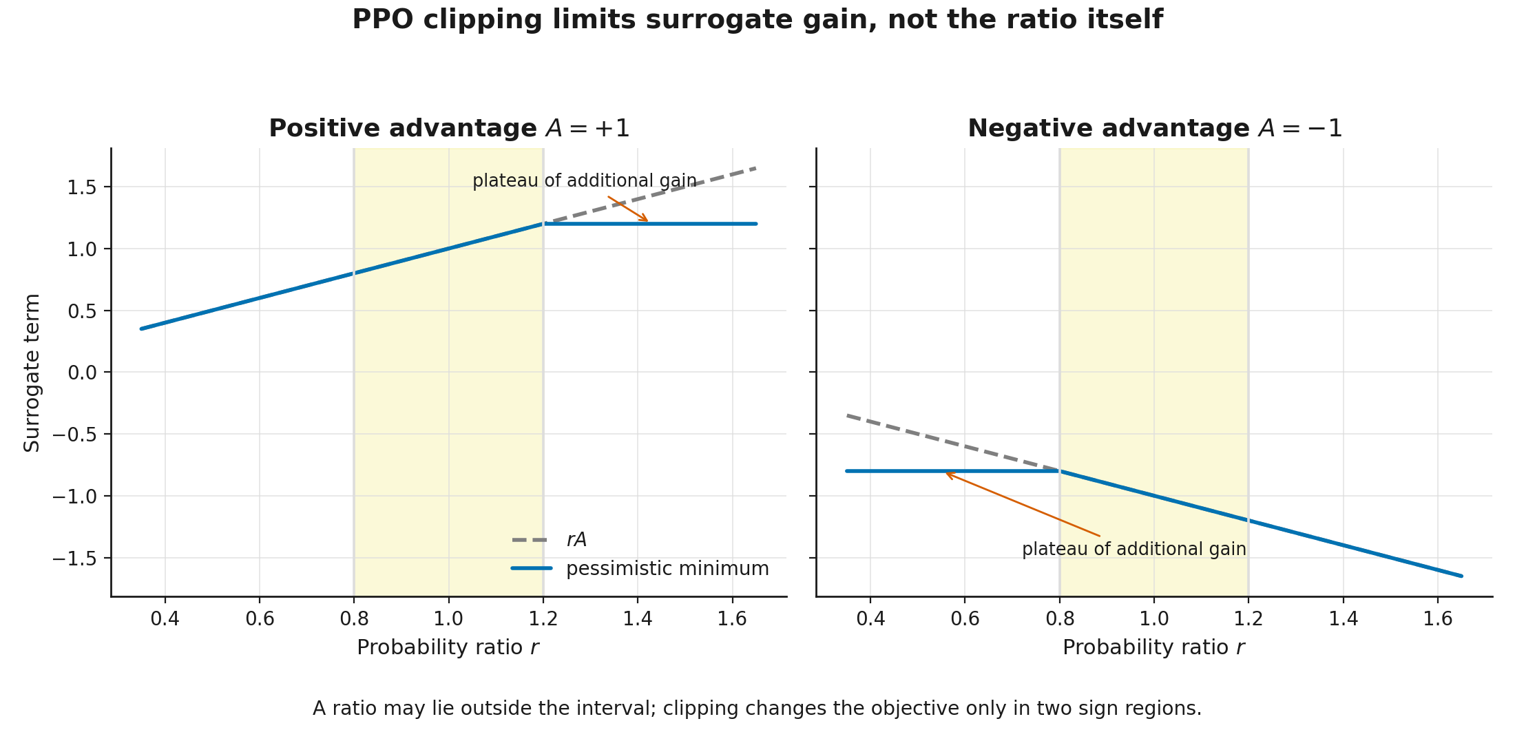
Step 4.4.3 — The clipped PPO objective
PPO's clipped objective is
The minimum forms a pessimistic version of the local gain.
For , making the action more likely is desirable. Increasing is rewarded only up to ; beyond that, further increase receives no additional objective gain. A fall below is still penalized.
For , making the action less likely is desirable. Decreasing is rewarded only down to ; below that, there is no additional gain. Increasing above remains fully penalized.
| Advantage sign | Ratio movement | Does the plateau activate? |
|---|---|---|
| excessive increase | yes | |
| excessive decrease | no | |
| excessive increase | no | |
| excessive decrease | yes |
Because of min, the fraction of ratios outside the interval and the fraction for which clipping actually changes the objective are different statistics.
Step 4.4.4 — The full loss and diagnostics
A typical implementation minimizes a combination of three terms:
Here is the critic loss, is policy entropy, and the coefficients set relative scale. Implementations may also clip value changes, normalize advantages, and stop an epoch when empirical KL becomes too large.
Useful diagnostics include:
- mean return and episode length;
- critic loss and explained variance;
- policy entropy;
- fraction of ratios outside ;
- fraction of samples where the clipped branch is actually the minimum;
- an empirical KL estimate under old-policy data;
- mean and standard deviation of advantages;
- gradient norm.
A numerically stable nonnegative sample expression is formed from each :
because . For a fixed state, with actions sampled from the old policy and the required support overlap,
The equality uses . A finite rollout batch satisfies that identity only approximately, so is a sample diagnostic—not an exact KL measurement and not a guarantee that the update stayed inside a trust region.
There is no universal “correct” clip fraction or KL value. Appropriate scales depend on model size, token aggregation, number of epochs, batch size, optimizer, and advantage quality. Diagnostics compare runs within a defined protocol; they are not magic certificates.
Step 4.4.5 — Why implementation details are part of the algorithm
The high-level PPO pseudocode is short, yet behavior depends strongly on:
- value-head initialization and scale;
- normalization of observations, rewards, and advantages;
- handling of termination and truncation;
- mini-batch shuffling order;
- epochs per rollout batch;
- learning-rate schedule;
- gradient-norm clipping;
- entropy bonus;
- numerical stability of log-probabilities;
- storing old log-probabilities before any update.
In the PPO and TRPO settings studied by the authors, these choices substantially changed results and sometimes explained differences previously attributed to the algorithms themselves. The conclusion is not that PPO is “not an algorithm.” Rather, a reproducible specification includes the data-collection, optimization, and evaluation protocol as well as the equation.
The notebook therefore has two modes. smoke validates shapes, masks, finite losses, and a short update cycle. full performs a complete training run and reports time and outcome statistics. One successful seed does not establish robustness; comparisons require multiple seeds and uncertainty intervals.
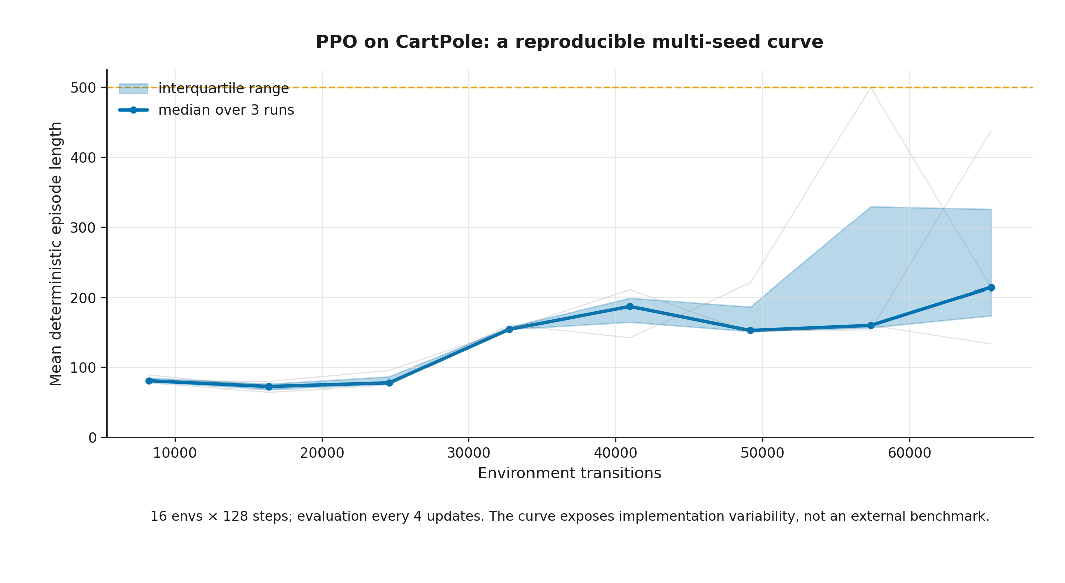
The figure is generated by the same implementation that trains the notebook policy. It demonstrates an auditable end-to-end loop; CartPole is not presented as evidence that PPO will behave the same way on LLMs.
Lesson 4.5. The bridge to LLM training
Lesson 4.5. The bridge to LLM training
- Sequence-level REINFORCE
- RLOO for several responses to one prompt
- Where group-relative policy optimization matches this picture
- One coefficient for every token does not solve credit assignment
- The module's final map
then 3 assessment steps
Step 4.5.1 — Sequence-level REINFORCE
For prompt and response
an autoregressive policy factorizes as
Therefore,
If a verifier returns one reward for the whole response, a practical masked estimate is
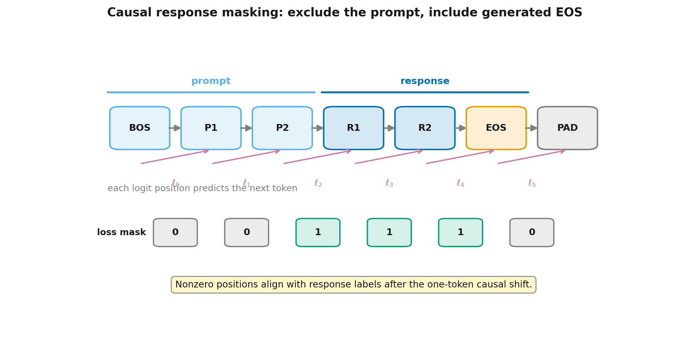
Set for generated response tokens, including a generated EOS token when it is present, and for prompt tokens, padding, and positions after EOS. In a causal language model, logits at position predict the token at position ; labels, selected log-probabilities, and the response mask must therefore be shifted together. A one-position error can silently train on prompt tokens or remove the first response token.
Optional model-interface deepening: tokenization, special tokens, and causal input-label alignment are developed in Modern LLMs, Module 2 “Tokenization and Embeddings” (modern_llms.module_02_tokenization). The present explanation is sufficient to implement the response mask; the cross-reference supplies the broader language-model context.
When the collected batch is reused by PPO, a local ratio can be formed at every valid response token:
With one whole-response advantage , a common tokenwise surrogate is
This is a local PPO surrogate, not the exact probability ratio of the complete trajectory. The exact sequence ratio is the product ; clipping every factor and clipping the product are different operations. An implementation must therefore name its reduction unit: all valid tokens in the batch, tokens averaged within each response, or responses averaged after token summation. Those choices weight length differently and generally define different objectives.
A non-differentiable reward is no obstacle: gradients flow through model log-probabilities. The same coefficient still weights the entire response, however. It says that the response as a whole was above or below its baseline; it does not identify which token supplied the proof, caused the error, or made a useful tool call.
Normalization must be explicit. Summing over tokens, averaging within each response, and averaging over every unmasked token in a batch assign different weight to short and long answers. A naturally sampled EOS and a forced max_tokens cutoff also have different semantics: in the latter case the response could have continued, so the reward rule and treatment of incompleteness belong in the task specification.
Finally, a penalty that depends directly on the current policy—such as a differentiable KL term—falls under the extended identity in Step 4.1.2. It must either enter the loss through its direct derivative or be deliberately inserted into a stop-gradient reward. Using both paths implicitly can double-count the term or optimize a different objective from the equation on the page.
Step 4.5.2 — RLOO for several responses to one prompt
Generate responses for one prompt, with rewards . RLOO defines
Its gradient estimate is
Advantages are measured relative to other responses for the same prompt, reducing sensitivity to prompt-to-prompt shifts in the baseline reward level. No separate critic is required. This is attractive when prompts can be repeated and responses generated in parallel.
The cost is generations per prompt. If all responses receive the same reward, the RLOO/REINFORCE term has zero advantages and supplies no update direction. That is a correct response to the absence of within-group signal, but it does not prove the policy is optimal: the verifier may simply be too coarse. Separate terms in the total loss—such as KL regularization, an entropy bonus, or an auxiliary objective—may still change the parameters.
Off-policy variants add sequence ratios or other corrections. Their stability depends on response length and on the distance between the collection and target policies.
Step 4.5.3 — Where group-relative policy optimization matches this picture
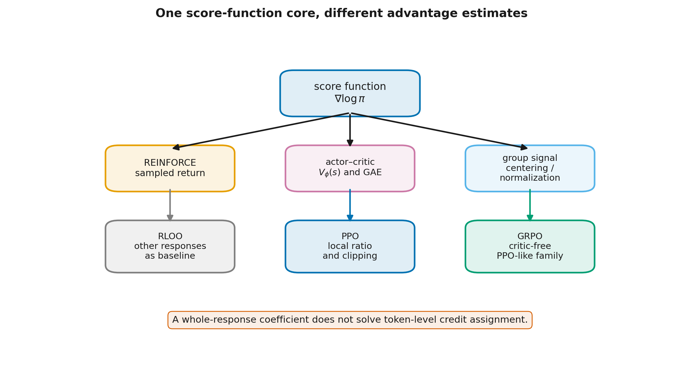
Group relative policy optimization (GRPO) also samples several responses to one prompt and forms relative advantages without a separate critic. RLOO and GRPO therefore share an important idea: compare responses within a group.
They are not identical.
The canonical GRPO formulation introduced in DeepSeekMath uses PPO-like probability ratios, a clipped surrogate, group centering and normalization of rewards, and regularization toward a reference policy. Later variants change the denominator, token aggregation, KL estimator, number of updates, and advantage construction.
Basic RLOO is a REINFORCE estimator with the current response excluded from the baseline mean. It need not include PPO clipping, division by group standard deviation, or a separate KL penalty.
The accurate map is:
- shared idea: multiple responses per prompt and a relative signal;
- RLOO: a leave-one-out baseline for whole-response REINFORCE;
- GRPO: a family of critic-free, PPO-like methods using group-relative estimates;
- Module 9 of this course: “RLVR and GRPO: Verifiable Reward, Group-Relative Estimation, and Stability” (
rl_llm.module_09_rlvr_grpo) — denominator choices, KL terms, token aggregation, and failure modes.
A broader architecture-level map of RLHF, DPO, RLOO, and GRPO is also available in Modern LLMs, Module 14 “Learning from Feedback: RLHF, DPO, RLOO, and GRPO” (modern_llms.module_12_preference_optimization). The present module remains self-contained and is the series’ canonical derivation of policy gradients and PPO.
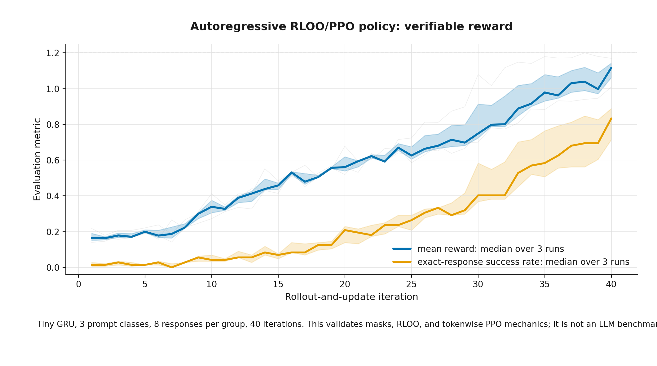
To keep this map from remaining purely algebraic, the module code trains a small autoregressive GRU policy on three prompt classes. Responses have variable length, EOS is genuinely sampled by the policy, prompt and padding positions are removed by the mask, RLOO advantages are built within each prompt group, and repeated PPO epochs use frozen old token log-probabilities with a clipped surrogate. The figure reports medians and interquartile ranges over three fixed runs. Improving verifiable reward checks agreement among those implementation contracts; it is not a language-quality benchmark and does not establish scaling behavior for large LLMs.
Step 4.5.4 — One coefficient for every token does not solve credit assignment
Suppose a response receives advantage . The simplest implementation creates a token matrix
for each valid response token and multiplies it by the token mask. This is convenient and gives the correct whole-response score-function objective:
But it does not solve credit assignment. Every sampled token receives the same sign and scale even though the true cause of reward may be local. Possible extensions include:
- intermediate verifiable rewards;
- process reward models;
- prefix value functions;
- higher-level action decomposition;
- counterfactual or search-based estimates;
- rewards for tool calls and environment states.
Each extension adds assumptions. A process reward may be denser but wrong; a value function may reduce variance but introduce bias; automatic step labels may reward superficial features.
The appropriately modest claim is conditional. Under on-policy sampling, with reward treated as fixed with respect to the optimization parameters and with an explicitly defined sum over correctly masked response tokens, whole-response REINFORCE estimates the gradient of expected whole-response reward. It still does not provide a local explanation of that reward. Reusing responses off-policy requires distribution-shift corrections, while length averaging, clipping, or parameter-dependent penalties define a different objective.
Step 4.5.5 — The module's final map
The module built one continuous chain:
- the log-derivative identity turns a gradient of an expectation into an expectation containing a score function;
- direct dependence on adds the integrand's own derivative to the score-function term;
- trajectory factorization leaves only parameterized components in the explicit derivative;
- causality replaces full return with reward-to-go;
- REINFORCE gives a simple but noisy estimator;
- a valid baseline reduces noise when it is independent of the current action;
- a critic approximates state value, while GAE mixes horizons and needs separate bootstrap and recursion masks;
- PPO reuses a rollout batch through a pessimistic local surrogate;
- RLOO uses other responses to the same prompt as a baseline group;
- GRPO shares the group idea but belongs to a broader PPO-like family.
The boundaries are just as important:
- removing environment dynamics from the explicit derivative does not remove the environment from the outcome;
- dropping the outer can change relative time weighting rather than merely rescale a gradient;
- is useful but not a universally variance-minimizing baseline;
- the same-group mean carries the finite-sample factor ;
- true termination, environment truncation, and a rollout boundary answer different questions;
- PPO clipping is not a hard trust region;
- one response-level reward does not solve token-level credit assignment;
- a correct response mask includes generated EOS, excludes the prompt, and follows the causal label shift;
- one successful learning curve does not establish implementation robustness.
Later modules use this foundation for preference-based training, verifiable rewards, and interaction with external environments. The full GRPO treatment is deliberately deferred to Module 9 “RLVR and GRPO: Verifiable Reward, Group-Relative Estimation, and Stability” (rl_llm.module_09_rlvr_grpo) so that this module can preserve a clean path from score functions to PPO.
Optional mathematical deepening: Information Theory for ML, Module 8 “Maximum entropy, exponential models, and KL regularization” (it_ml.module_08_maxent_kl_policy) — the variational derivation of KL-regularized policies, Gibbs form, and the normalizing constant.
Architecture context: Modern LLMs, Module 14 “Learning from Feedback: RLHF, DPO, RLOO, and GRPO” (modern_llms.module_12_preference_optimization) — how these methods fit into an end-to-end LLM post-training pipeline. Neither reference is required to understand this module.
Practice route
- REINFORCE variance and the effect of baselines;
- GAE telescoping and distinct masks for terminals, truncations, and buffer boundaries;
- a complete PPO loop on a self-contained CartPole environment;
- multi-seed evaluation rather than a single favorable trajectory;
- an autoregressive example with response masks, EOS, group advantages, and a clipped objective.
The learning platform adds 32 exercises—20 on the core route and 12 optional platform extensions—with worked solutions revealed after an attempt.
CPU is sufficient. smoke runs a short end-to-end validation; full increases rollout and seed counts. The resulting curves are computations made by course code under the stated protocol, not external benchmarks.
Sources and further reading route
- Williams, “Simple Statistical Gradient-Following Algorithms for Connectionist Reinforcement Learning” — the original REINFORCE paper; it supports the historical and algorithmic account in Lesson 4.1 but does not promise low variance.
- Sutton, McAllester, Singh, and Mansour, “Policy Gradient Methods for Reinforcement Learning with Function Approximation” — the policy-gradient theorem with function approximation; constants depend on the objective and occupancy convention.
- Schulman et al., “High-Dimensional Continuous Control Using Generalized Advantage Estimation” — GAE and its bias–variance logic. The mask discussion in this module also uses modern environment API semantics.
- Schulman et al., “Trust Region Policy Optimization” — trust-region motivation and the limits of the theoretical guarantee.
- Schulman et al., “Proximal Policy Optimization Algorithms” — the primary PPO specification and clipped surrogate; clipping is not stated as a strict KL guarantee.
- Engstrom et al., “Implementation Matters in Deep Policy Gradients” — empirical evidence that implementation protocol belongs in the experimental specification; conclusions are tied to the studied benchmarks.
- Farama Foundation, “Handling Time Limits” — official semantics for
terminatedandtruncated; rollout-buffer boundaries are separated further in this module. - Ahmadian et al., “Back to Basics: Revisiting REINFORCE Style Optimization for Learning from Human Feedback in LLMs” — RLOO and sequence-level REINFORCE for LLM post-training.
- Shao et al., “DeepSeekMath” — the primary GRPO formulation; later variants should not be projected backward onto every detail of that paper.
Module_4_Sources.md contains the full claim registry, evidence classes, and scope limits.